
ICON Training - Hands-on Session
Exercise 6.3: ICON ComIn, Part III#
The ICON Community Interface (ComIn) enables the integration of plugins which is a flexible way to extend the code with your own routines and variables at run-time.
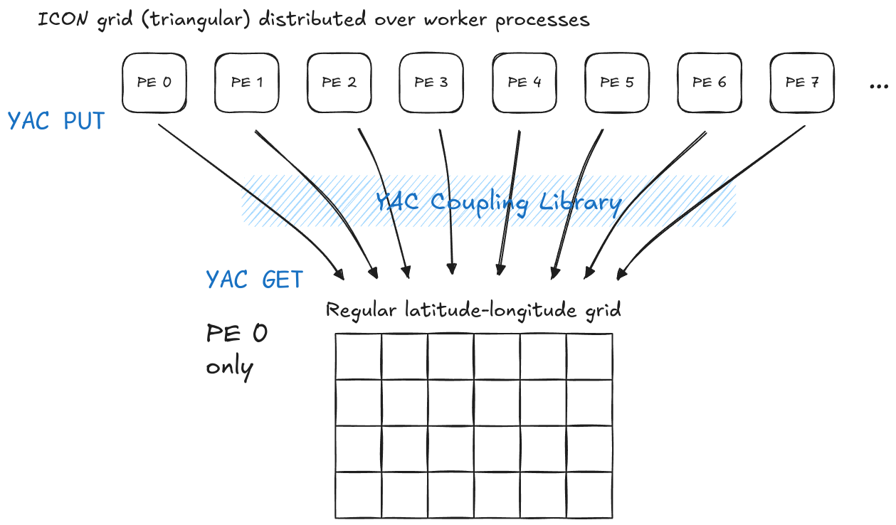
Step P3: In the final step, we learn how to use the coupling library YAC in a plugin to interpolate fields from the ICON unstructured grid onto a custom lat-lon grid, and then visualize the interpolated fields.
Step P3: Using YAC in ComIn plugin for interpolation#
|
Exercise:
In this exercise, we will develop the plugin step by step. Some parts will be provided, and you will be asked to implement the necessary missing components:
Access the surface pressure ( |
|
Step-by-step writing ComIn plugin#
In this notebook, we will append Jupyter notebook code cells to the initially empty file scripts/comin_plugin_P3.py, step by step. This will happen automatically as we run the cells. To do this, we’ll define a custom Jupyter cell magic command in append_magic.py.
%load_ext append_magic
First steps:
We need to import the necessary packages, most importantly,
yacandcomin.We get the neccessary descriptive data.
We query the YAC instance ID. This is the predefined identifier used to reference the YAC instance for defining components, grids, and times in the coupling framework.
%%append_to_script scripts/comin_plugin_P3.py --reset

from yac import (
    YAC, Reg2dGrid, Location, Field, TimeUnit, Reduction,
    InterpolationStack, NNNReductionType, UnstructuredGrid
)
import comin
import numpy as np
import matplotlib.pyplot as plt


# === GET DESCRIPTIVE DATA STRUCTURE ===

domain = comin.descrdata_get_domain(1) # DOMAIN 1
glob = comin.descrdata_get_global()
rank = comin.parallel_get_host_mpi_rank()

assert glob.yac_instance_id != -1, "The host-model is not configured with YAC"
yac = YAC.from_id(glob.yac_instance_id)
We then define the source grid and component. YAC components are the individual Earth system model components - such as atmosphere, ocean, or an output writer - that are coupled together to exchange data fields through the YAC library.
The source component will be based on ICON’s computational grid and the following code snippets show how to define such an unstructured mesh with the YAC coupler.
%%append_to_script scripts/comin_plugin_P3.py

# === DEFINE SOURCE GRID AND COMPONENT ===

source_component = yac.predef_comp("comin_example_source")

ncells = domain.cells.ncells
nverts = domain.verts.nverts

# the "connectivity" field contains the three vertices for each cell:
connectivity = (np.asarray(domain.cells.vertex_blk) - 1) * glob.nproma + (
    np.asarray(domain.cells.vertex_idx) - 1
)

# We also provide the geographical coordinates for each vertex.
# Please note that we need to specify the 'order=F' argument
# because Fortran (ICON) uses column-major ordering.
icon_grid = UnstructuredGrid(
    "icon_grid",
    np.ones(domain.cells.ncells) * 3,
    np.ravel(domain.verts.vlon, order='F')[: domain.verts.nverts],
    np.ravel(domain.verts.vlat, order='F')[: domain.verts.nverts],
    np.ravel(np.swapaxes(connectivity, 0, 1))[: 3 * domain.cells.ncells],
)

# "def_points": This method is used to specify the locations (such as corners,
# centers, or edges) of grid points for coupling fields between components.
icon_cell_centers = icon_grid.def_points(
    Location.CELL,
    np.ravel(domain.cells.clon)[:ncells],
    np.ravel(domain.cells.clat)[:ncells],
)
Some hints:
- Grid coordinates are given in radians (use `np.deg2rad`))
- The lat and lon coordinates are (44.1, 57.5), and (1.0, 16.6) respectively
%%append_to_script scripts/comin_plugin_P3.py

#write your code here
Solution
if rank == 0:
    target_component = yac.predef_comp("comin_example_target")

    vlon = np.deg2rad(np.arange(1.0, 16.6 + 0.001, 0.05))
    vlat = np.deg2rad(np.arange(44.1, 57.5 + 0.001, 0.05))
    grid = Reg2dGrid("example_grid", vlon, vlat, cyclic=(True, False))
    cell_centers = grid.def_points(
        Location.CELL,
        vlon + 0.5 * (vlon[1] - vlon[0]),
        vlat[:-1] + 0.5 * (vlat[1] - vlat[0]),
    )
Now, we access the variable pres_sfc in the secondary constructor, in a similar way to the previous exercises P1 and P2.
%%append_to_script scripts/comin_plugin_P3.py

@comin.EP_SECONDARY_CONSTRUCTOR
def secondary_constructor():
    global comin_pres_sfc
    comin_pres_sfc = comin.var_get(
        [comin.EP_ATM_WRITE_OUTPUT_BEFORE],
        ("pres_sfc", 1),
        comin.COMIN_FLAG_READ
    )
%%append_to_script scripts/comin_plugin_P3.py

@comin.EP_ATM_YAC_DEFCOMP_AFTER
def define_fields():
    global yac_pres_sfc_target, yac_pres_sfc_source

    step = str(int(comin.descrdata_get_timesteplength(1)))
    yac_pres_sfc_source = Field.create(
        "pres_sfc", source_component, icon_cell_centers, 1, step, TimeUnit.SECOND,
    )
    if rank == 0:

        # >>>>
        # TODO: Define the target field here
        # <<<<

        nnn = InterpolationStack()
        nnn.add_nnn(NNNReductionType.AVG, n=1, scale=1.0, max_search_distance=0.0)
        yac.def_couple(
            "comin_example_source",
            "icon_grid",
            "pres_sfc",
            #ToDo,
            #ToDo,
            #ToDo,
            step,
            TimeUnit.SECOND,
            Reduction.TIME_NONE,
            nnn,
        )
Solution
    if rank == 0:
        yac_pres_sfc_target = Field.create(
            "pres_sfc", target_component, cell_centers, 1, step, TimeUnit.SECOND,
        )
        nnn = InterpolationStack()
        nnn.add_nnn(NNNReductionType.AVG, n=1, scale=1.0, max_search_distance=0.0)
        yac.def_couple(
            "comin_example_source",
            "icon_grid",
            "pres_sfc",
            "comin_example_target",
            "example_grid",
            "pres_sfc",
            step,
            TimeUnit.SECOND,
            Reduction.TIME_NONE,
            nnn,
        )
Finally, we put the source field on the source grid and get the target field on the target grid.
%%append_to_script scripts/comin_plugin_P3.py

#=== HELPER FUNCTION ====
import isodate

def is_time_to_plot(interval_iso):
    """Check if the current time is at the start of a given interval."""
    interval = comin.descrdata_get_simulation_interval()
    exp_start = np.datetime64(interval.exp_start)
    current_time = np.datetime64(comin.current_get_datetime())
    interval_ns = int(isodate.parse_duration(interval_iso).total_seconds() * 1e9)
    elapsed_ns = (current_time - exp_start).astype('timedelta64[ns]').astype(int)
    return (elapsed_ns % interval_ns) == 0


## === PUT and GET fields (Partially Given) ===

@comin.EP_ATM_TIMELOOP_END
def process():
    yac_pres_sfc_source.put(np.ravel(comin_pres_sfc)[: domain.cells.ncells])
    if rank == 0:

        # >>>>
        # TODO: get the field via a call to the YAC library
        # <<<<

        # Plot the interpolated field every 1 hour
        if is_time_to_plot("PT1H"):
            plt.imshow(np.reshape(data, [vlat.shape[0]-1, vlon.shape[0]]))
            filename = f"pres_sfc_{comin.current_get_datetime()}.png"
            print(filename)
            plt.savefig(filename)
Solution
data, info = yac_pres_sfc_target.get()
At this point, you have completed your plugin. Now, let’s run the ICON!
Running the ICON model#
import os
import subprocess

user = os.environ['USER']
home = os.environ['HOME']
scratchdir = f"/scratch/{user[0]}/{user}"
icondir = f"/pool/data/ICON/ICON_training/icon"
expdir = f"{scratchdir}/exercise_comin/P3"
%env ICONDIR={icondir}
%env EXPDIR={expdir}
%env SCRATCHDIR={scratchdir}
Run the setup script which generates the namelists, output directory etc.:
!bash $HOME/icon-training-scripts/exercise_comin/prepared/prepare_icon_run.sh
As in the previous exercises, we have to append the plugin block to the ICON namelist settings:
with open(f"{expdir}/NAMELIST_ICON", 'a') as f:
    f.write(f"""&comin_nml
   plugin_list(1)%name           = "comin_plugin"
   plugin_list(1)%plugin_library = "{icondir}/build/externals/comin/build/plugins/python_adapter/libpython_adapter.so"
   plugin_list(1)%options        = "{home}/icon-training-scripts/exercise_comin/scripts/comin_plugin_P3.py"
/
""")
We have to append the coupling_mode_nml block to the ICON namelist settings so the yac would initialize by ICON:
with open(f"{expdir}/NAMELIST_ICON", 'a') as f:
    f.write(f"""&coupling_mode_nml
    coupled_to_output = .TRUE.
/
""")
Submit the job. The job will run for approximately 2:30 minutes.
!cd $EXPDIR && sbatch --account=$SLURM_JOB_ACCOUNT --export=ICONDIR $EXPDIR/icon-lam.sbatch
!squeue -u $USER
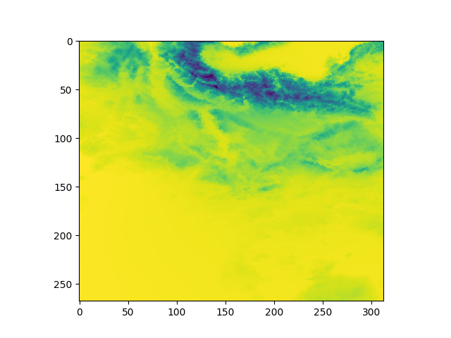
Display one of the generated output images:
from IPython.display import Image, display
path = f"{expdir}/pres_sfc_2021-07-14T12:00:00.000.png"
display(Image(filename=path))
Solution
The resulting plot pres_sfc_2021-07-14T12:00:00.000.png looks like this:
Congratulations! You have successfully completed Exercise 6, Part III.
By the way: Further examples of the ICON Community Interface (ComIn) in Jupyter can be found at https://gitlab.dkrz.de/icon-comin/comin-training-exercise. ComIn also comes with several example plugins that demonstrate its usage with plugins written in Fortran and C/C++, which can be found at https://icon-comin.gitlab-pages.dkrz.de/comin/.
Further Reading and Resources#
-
ICON Tutorial, Ch. 9: https://www.dwd.de/DE/leistungen/nwv_icon_tutorial/nwv_icon_tutorial.html
A new draft version of the ICON Tutorial is available here: https://icon-training-2025-scripts-rendering-cc74a6.gitlab-pages.dkrz.de/index.html. It is currently being finalized and will be published soon. - Documentation on the ICON ComIn project website: https://gitlab.dkrz.de/icon-comin/comin/-/blob/master/doc/icon_comin_doc.md?ref_type=heads
- Python API description for ICON ComIn: https://gitlab.dkrz.de/icon-comin/comin/-/blob/master/doc/comin_python_api.md?ref_type=head
Author info: Deutscher Wetterdienst (DWD) 2025 :: icon@dwd.de. For a full list of contributors, see CONTRIBUTING in the root directory. License info: see LICENSE file.