ICON Training - Hands-on Session

Exercise 0: Getting familiar with the Jupyter Notebooks#

We begin with JupyterLab, a web-based interactive computational environment. This step-by-step exercise will familiarize you with the basic functionalities of the “Levante” JupyterLab server.

The exercise covers the following introductory topics:

the JupyterLab user interface,
the Slurm job scheduler,
the Levante high-performance computing system and its file systems.

To get the most out of this tutorial you should already have some knowledge about Linux/UNIX and batch systems for computer clusters.

Starting the JupyterLab server#

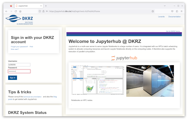
First, open the web site https://jupyterhub.dkrz.de and enter your username and the corresponding password on the start page of the JupyterLab portal. If you do not yet have a DKRZ account for Levante, please contact the course instructors.

This opens a web page (“Hub Control Panel”) where the details of the JupyterLab server can be entered. For this training course, we recommend selecting the “Preset” settings.

Before the JupyterLab server can actually be started, the account name must be entered in the form. This account is used for billing the HPC resources used. The server itself is started on one of the non-exlusive, interactive nodes of the cluster.

exercise_0_2.marker.png

Copying the course notebooks, Levante file systems#

The first thing we need to do for this course is to install the Jupyter notebooks containing the exercises and the course material - including the icon_exercise_zero.ipynb notebook you are currently viewing. We also provide a brief introduction to the Levante HPC file systems, with more details available in the reference given below. It is recommended that you follow the suggested directory structure, as the path configurations within the notebooks depend on this layout for proper operation.

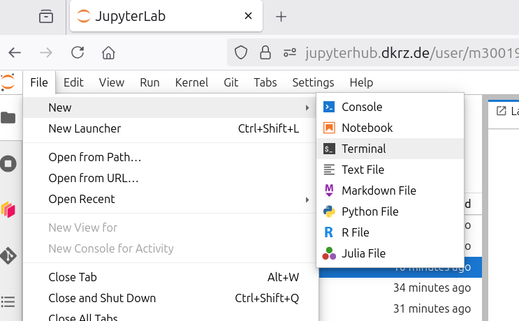
Open an interactive terminal with your JupyterLab session.

The course notebooks are stored in a public Gitlab repository https://gitlab.dkrz.de/icon-training/icon-training-2025-scripts. Please clone this repository (using the terminal) to your home directory, generating a directory icon-training-scripts:

cd $HOME
git clone https://gitlab.dkrz.de/icon-training/icon-training-2025-scripts.git icon-training-scripts

The $HOME directory is used to store shell setup files, source code, and scripts. However, it is not intended for the temporary storage or processing of large amounts of data. Therefore, all our experiment output will be written to the SCRATCH space, which can be accessed via $SCRATCHDIR after defining

export SCRATCHDIR=/scratch/${USER::1}/$USER

In other words, the path name is /scratch/, followed by the first letter of your user ID and the user-specific subdirectory named userID, for example: /scratch/k/k1234.

For the sake of time, the ICON binary has been pre-built for you. It is located in the /pool/data/ICON/ICON_training/icon folder. The precise instructions for configuring and building the ICON executable will only be discussed in later exercises, specifically “Programming ICON”, where you will learn to modify the Fortran code itself.

Basics of the JupyterLab user interface#

The screenshot below shows JupyterLab’s main work area (1), which is the central part of the interface where you interact with your documents and activities. Other elements of the web environment are the collapsible left sidebar (2), and a menu bar (3).

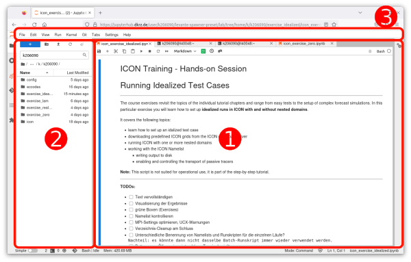
The recipes for running the ICON forecasts and for monitoring the cluster are organized as JupyterLab notebooks. These files (with the extension *.ipynb) combine description text, commands and the respective output. The filename is visible as the title of the active tab at the top of the main work area.

Jupyter notebooks are composed of cells. A cell is a block of text to be displayed in the notebook or code to be executed, like the following:

ls -l /home

You can run the above code cell using Shift-Enter or by pressing the button in the toolbar:

Exercise: Run the above code cell.

The ICON notebooks mostly contain shell commands, but other Jupyter notebooks can also execute Python code. The “computational engine” behind each notebook is called the kernel. Using the wrong kernel sometimes leads to confusing error messages, e.g. when executing the following code:

whoami

You can select the kernel at the top right of the working area:

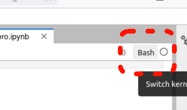
Exercise: Switch to the bash kernel and repeat the execution of the previous cell.

By default, the left sidebar is filled by a file browser. If you hover the mouse pointer over the folder icon at the very top, you will see the name of the current directory.

You can upload and download files manually via the file browser (context menu). Of course, you could also simply use an SSH client software and scp.

Slurm batch jobs#

In the next step, we will embed a command into a Slurm batch job script and submit the job to the cluster.

The SLURM sinfo command lists all partitions and nodes managed by SLURM.

sinfo

        PARTITION   AVAIL  TIMELIMIT  NODES  STATE NODELIST
visualize      up 2-00:00:00      1  alloc lg1
visualize      up 2-00:00:00      3   idle lg[0,2-3]
gpu            up   12:00:00      4   resv l[50018,50033,50048,50175]
gpu            up   12:00:00     13   plnd l[50109,50112,50115,50118,50121,50124,50130,50133,50136,50139,50142,50145,50148]
gpu            up   12:00:00      4 drain$ l[40363,50000,50063,50072]
gpu            up   12:00:00     24    mix l[50003,50006,50009,50012,50015,50021,50024,50027,50030,50036,50039,50045,50051,50057,50066,50069,50075,50078,50081,50100,50103,50106,50127,50154]
gpu            up   12:00:00     15  alloc l[40360,40366,40369,50042,50054,50060,50151,50157,50160,50163,50166,50169,50172,50178,50181]
compute        up    8:00:00    100   plnd l[20400,20405,20408,20410-20416,20421-20429,20439-20441,20444,20449,20451-20452,20455-20457,20500-20503,20505-20514,20517-20518,20520-20531,20533-20539,20542-20547,20648,20654-20662,20666,20673-20690,20692]
compute        up    8:00:00      8   comp l[10115-10122]
compute        up    8:00:00      8   resv l[10028,10567,20348-20349,20351,20353,20356-20357]
compute        up    8:00:00   2637  alloc l[10000-10027,10029-10058,10060-10095,10100-10114,10123-10158,10160-10195,10200-10258,10260-10295,10300,10309-10322,10324-10395,10400-10491,10500-10566,10568-10595,10608,10626-10627,10636-10695,10700-10787,10789-10795,20000-20095,20100-20195,20200-20295,20300-20347,20350,20352,20354-20355,20358-20395,20401-20404,20406-20407,20409,20417-20420,20430-20438,20442-20443,20445-20448,20450,20453-20454,20461-20463,20471,20504,20515-20516,20519,20532,20540-20541,20548-20595,20600-20647,20649-20653,20663-20665,20667-20672,20691,20693-20695,30000-30095,30100-30195,30200-30295,30300-30316,30318-30339,30344-30395,30400-30487,30489-30495,30500-30553,30600-30637,30639-30689,30691-30695,30700-30795,40021-40047,40072-40083,40090-40095,40100-40183,40190-40192,40194-40195,40200-40283,40287-40295,40300-40347,40349-40359,40400-40459,40500-40571,40577,40580,40582-40585,40592-40595,40600-40683,40687-40695,50200-50295,50300-50333,50335-50359,50369-50371]
compute        up    8:00:00    184   idle l[10301-10308,10323,10492-10495,10600-10607,10609-10625,10628-10635,10788,20458-20460,20464-20470,20472-20495,30317,30340-30343,30488,30554-30595,30638,30690,40193,40348,40460-40495,40572-40576,40578-40579,40581,40586-40591,50334]
shared         up 7-00:00:00      2   resv l[10028,10567]
shared         up 7-00:00:00     16    mix l[40000-40010,40012-40014,40016,40020]
shared         up 7-00:00:00      3  alloc l[40011,40015,40017]
shared         up 7-00:00:00      2   idle l[40018-40019]
interactive    up   12:00:00      5    mix l[40048-40050,40055,40057]
interactive    up   12:00:00      6  alloc l[40072-40077]
interactive    up   12:00:00     19   idle l[40051-40054,40056,40058-40071]
daki           up 14-00:00:0      3   idle l[50187,50190,50193]
vader          up 2-00:00:00      3   idle vader[1-3]
gpu-devel      up      30:00      3   idle vader[1-3]
dolpung        up   12:00:00      1  inval l50437
dolpung        up   12:00:00      1 drain~ l50436
dolpung        up   12:00:00      1    mix l50432
dolpung        up   12:00:00     41   resv l[50400-50431,50433-50435,50438-50443]

We can make use of the fact that the file systems (home directory, work and scratch) are accessible by all cluster nodes. The test program is the following script:

cat > $HOME/test.py <<EOF
import matplotlib.pyplot as plt
import xarray as xr
import cartopy.crs as ccrs
import numpy as np

ds = xr.open_dataset('/pool/data/ICON/ICON_training/icon_grid_0012_R02B04_G.nc')
lon = np.rad2deg(ds["cell_area"].clon)
lat = np.rad2deg(ds["cell_area"].clat)
ca = ds["cell_area"]

proj    = ccrs.PlateCarree()
x, y, z = proj.transform_points(proj, lon, lat).T
ax      = plt.axes(projection=ccrs.Orthographic())
ax.set_global()
plt.tricontourf(x, y, ca, transform=proj)

plt.savefig('test.png')

EOF

Launching this script on a single node will be sufficient. We therefore use the shared queue, intended for serial jobs.

This setting is specified with directives (SBATCH) in the job header, see, e.g., here for a comprehensive table.

Exercise: Complete the SBATCH options with the above information.

cat > $HOME/test.sbatch << 'EOF'
#!/bin/bash
#SBATCH --job-name=testjob
#SBATCH --partition=????????     # Specify partition name
#SBATCH --output=slurm.%j.out
#SBATCH --time=00:30:00

export NUMEXPR_MAX_THREADS=2
module load python3

python3 $HOME/test.py

################################
sleep 500

EOF

Solution

#SBATCH --partition=shared

Finally, we submit the batch job . The sbatch command will return immediately, resulting in a batch job ID. The --account=$SLURM_JOB_ACCOUNT option tells Slurm to charge the job to the account specified by the environment variable $SLURM_JOB_ACCOUNT (e.g., bb1234), allowing you to dynamically use the account assigned to your session or project.

sbatch --account=$SLURM_JOB_ACCOUNT $HOME/test.sbatch

Batch job monitoring#

While waiting for our test job to launch, we can monitor the cluster status. The squeue command reports the state of running and pending jobs.

Exercise: Execute the squeue command. Hint: The output gets shorter when specifying the user ID.

Solution

squeue -u $USER

The squeue command yields different status codes which are listed, for example, here. The most relevant for the ICON cluster are

Abbreviation	Job state	Description
`PD`	Pending	Job is awaiting resource allocation.
`R`	Running	application is running
`CG`	Completing	Job is in the process of completing. Some processes on some nodes may still be active.

Interactive Linux terminal in JupyterLab#

Open an interactive Linux terminal by clicking the following button:

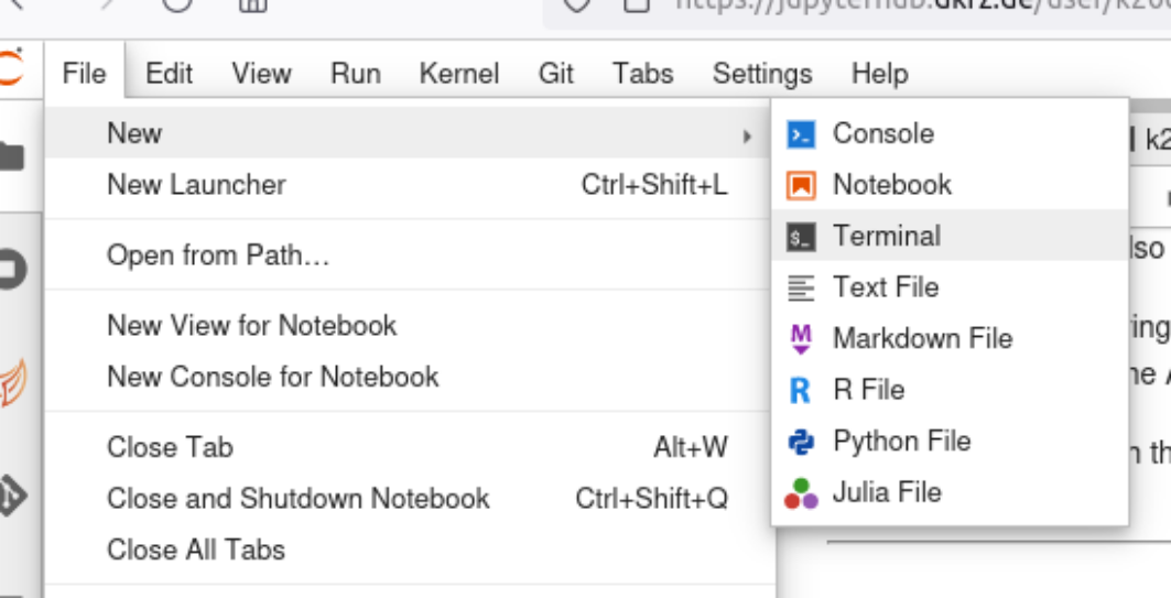
In general, to open an interactive Linux terminal start the launcher by pressing: CRTL+SHIFT+L (then click the terminal icon) or via the “File” menu:

Of course, the above squeue command can also be executed interactively in the terminal.

Aborting Slurm jobs#

The plotting batch job above intentionally included a sleep command so that the job would not exit immediately after the graph was created. This way we get a chance to practice terminating running Slurm jobs.

First, let’s repeat the squeue command to make sure the batch job is still running. This also provides an easy way to determine the job ID.

squeue

Exercise: Execute the command scancel <jobid> on the login node to abort the running batch job. Make sure afterwards (using squeue) that the job has actually been finished!

<your answer>

Solution

scancel <jobID>

The resulting grid plot looks like this:
../../_images/test.png

Final remark: Of course, you can also monitor the queue status using a Python kernel in a Jupyter notebook. We have prepared a demonstration script, squeue.ipynb, showing how to do this.

Congratulations! You have reached the end of this exercise! - To be continued!

Exercise 0: Getting familiar with the Jupyter Notebooks

Contents

ICON Training - Hands-on Session

Exercise 0: Getting familiar with the Jupyter Notebooks#

Starting the JupyterLab server#

Copying the course notebooks, Levante file systems#

Basics of the JupyterLab user interface#

Slurm batch jobs#

Batch job monitoring#

Interactive Linux terminal in JupyterLab#

Aborting Slurm jobs#

Further Reading and Resources#