
ICON Training - Hands-on Session
Exercise 3: Pre-Processing for ICON#
This step-by-step exercise will familiarize you with the necessary input data for the ICON model. We will prepare initial and boundary data for a limited area model run (ICON-LAM).
In detail, we will cover the following topics:
grids and external parameters
processing raw input data sets into initial and boundary data
We assume that the students are familiar with the contents of the basic exercises (Jupyter, Slurm, namelists).
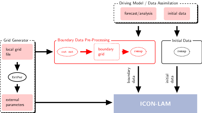
Overview#
Let’s start with a short examination of the necessary input data files. Later on we will generate (parts of) this data with the help of the Climate Data Operators (CDO). Detailed information on the datasets can be found in Chapter 2 of the ICON manual, see the link at the bottom of the page).
The following illustration gives an overview of the different building blocks.
First, we link the directory which contains some example files:
export SCRATCHDIR=/scratch/${USER::1}/$USER
cd $SCRATCHDIR
ln -sf /pool/data/ICON/ICON_training/test/example_data/ .
export EXAMPLEDIR=$SCRATCHDIR/example_data
The subdirectories therein point to
const: LAM grid data and external parameters
(see the block on the left in the above illustration)raw_data: the initial and boundary data retrieved from DWD’s database (see the block at the top of the illustration)pre_data: pre-processed initial and boundary data
(see the block in the middle of the figure)
<shell command>
Solution
The lateral boundary data reduces proportionally to the forecast time span.
Megabytes:
148M for 20210714 + 12 for 2021071500 instead of 294M total
cd $EXAMPLEDIR
du -ch ./raw_data/*20210714*
du -ch ./raw_data/*
pamore commands to retrieve these data? (Hint: see the ICON Manual. A link to the manual is provided in the References section at the end of this Jupyter notebook).
Solution
Initial data: pamore -d 2021071400 -hstart 0 -hstop 0 -lt a -model iglo -iglo_startdata_0
Boundary data: pamore -d 2021071400 -hstart 0 -hstop 48 -hinc 2 -model iglo -hindcast_ilam
Grids and external parameters#
In order to run the ICON model, it is necessary to load the horizontal grid information as an input parameter. This information is stored within so-called grid files. Additionally, external parameter fields describe properties of the Earth’s surface and atmosphere like the topography and the land-sea mask. Of course, we have already encountered these files in the previous exercises; now let’s take another closer look.
Grid files#
Providing the grid files is a one-time process. It only needs to be repeated if the model setup changes. Similarly, for the external parameters there are updates only at longer intervals, for example when updated raw data sets become available.
For fixed domain sizes and resolutions a list of grid files has been pre-built for the ICON model together with the corresponding external parameters.
Custom grid files can be generated through an online grid generator tool, see the References section below.
ICON data files do not completely contain the description of the underlying grid. To answer the question “Which grid file is related to my simulation data?”, users may compare the horizontal grid UUID, a non-human-readable sequence of numbers which is sort of a fingerprint attribute.
export GRIDFILENAME=$EXAMPLEDIR/const/iconR3B08_DOM01.nc
uuidOfHGrid in the grid file. To this end, display the NetCDF file header with the `ncdump` utility. The `ncdump` tool generates a text representation of a NetCDF file and is included in the netcdf-c module.
module load netcdf-c

<shell command>
Solution
module load netcdf-c
ncdump -h $GRIDFILENAME | grep uuidOfHGrid
For ICON grid files the following nomenclature has been established: In general, by RnBk we denote a grid that originates from an icosahedron whose edges have been initially divided into n parts, followed by k subsequent edge bisections.

With the information about n and k, the effective mesh size of a global grid can be estimated as
\( \overline{\Delta x} \approx 5050/(n\,2^k) \quad [\mathrm{km}]\,. \)
ncdump -h output for the grid file above. Find out about the root subdivision (grid_root) and the grid (bisection) level to estimate the mesh size.
<shell command>
Solution
module load netcdf-c
ncdump -h $GRIDFILENAME | grep -E 'grid_level|grid_root'

python3 - << EOF
n = 3 # grid_root
k = 8 # grid_level

mesh_size = 5050/(n * 2**k) # [km]
print(f"estimated mesh size: {mesh_size} km");
EOF
External parameter files#
Similar to the grid information, the ICON model reads its external parameters, e.g. the topography and the land-sea mask, from a NetCDF file.
export EXTPARFILENAME=$EXAMPLEDIR/const/external_parameter_icon_dom1_DOM01_tiles.nc
Solution
ncdump -h $EXTPARFILENAME | grep uuid # uuidOfHGrid attribute matches
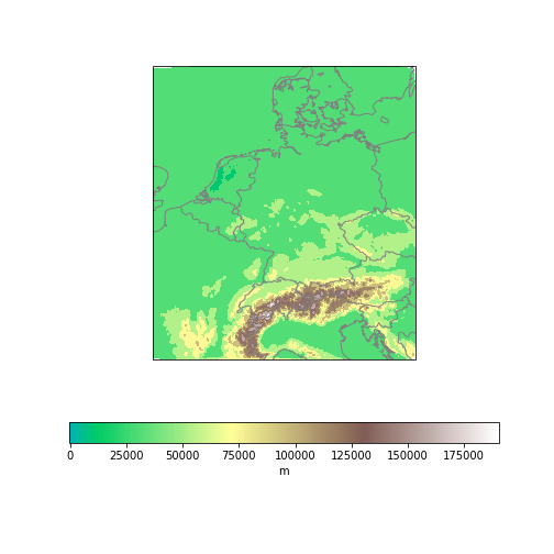
Among the various constant data, the field topography_c contains the geometric height of the earth’s surface above sea level. We will visualize the topography with the plot script scripts/icon_exercise_prepare_lam_plot_hsurf.ipynb.
<shell command>
This should generate a bitmap file HSURF.png; please check this by opening the image via the file browser. It should look like the following plot:
Raw input data sets#
Usually, the ICON limited area runs are driven by input data originating from DWD’s operational NWP process chain, see here for a summary description. These GRIB2 formatted raw data sets contain the so-called initialized analysis which means that the first guess and analysis fields have already been merged.
Before the data is delivered through DWD’s Automatic File Distribution (AFD) service, a data extraction of the global forecast data is performed. This step reduces the raw data to a subregion which roughly covers the limited area domain, while retaining the same mesh resolution as DWD’s global driving model.
Based on the above information on the local grid, we can (roughly) estimate the number of required raw data grid cells for the subregion. Currently, DWD's deterministic global forecast has a mesh size of roughly 13km. Estimate the number of grid cells that would need to be extracted from the DWD dataset.
<shell command>
Solution
calculate the factor between the mesh sizes: 13/6.5 = 2
(or we can also use the exact factor 2 when we know that the global DWD grid is anR03B07grid).get the
ncdump -hinfo on the local cell number:ncdump -h const/iconR3B08_DOM01.nc | grep cell(37488)calculate an estimate:
37488 / 2^2(9372)this is a rough estimate and a lower bound, the cut-out area usually contains significantly more cells
module load netcdf-c
ncdump -h $EXAMPLEDIR/const/iconR3B08_DOM01.nc | grep -m 1 cell

python3 - << EOF
mesh_size_global = 13.0
mesh_size_local   = 6.5
cell = 37488

factor = mesh_size_global/mesh_size_local
raw_cell = cell/factor**2

print("factor   =",factor)
print("raw_cell =",raw_cell);
EOF
At this point, we shortly introduce the grib_ls command, which is a basic command-line tool for displaying GRIB2 data. It is included in the ecCodes library and tools.
grib_ls tool on one of the raw input data sets and determine the number of levels. In ICON levels are ordered top-down such that the record with the largest level index corresponds to the level which is near the surface.
<shell command>
Solution
The dataset contains 90 levels of the global model, which differs from the ICON-LAM setup in the next hands-on exercise. Therefore, a vertical interpolation step is required as part of the ICON model initialization.
module load eccodes
export ECCODES_DEFINITION_PATH=/pool/data/ICON/ICON_training/eccodes/definitions.edzw-2.27.0-1:$ECCODES_DEFINITION_PATH

grib_ls -w shortName=T $EXAMPLEDIR/raw_data/init_ML_20210714T000000Z.grb
The grib_ls utility also accepts an option -P <key> for displaying additional metadata key.
grib_ls tool once more and find out about the `localCreationDateYear`, `localCreationDateMonth`, `localCreationDateDay` of the initial data set file in the raw input data set.
<shell command>
Solution
module load eccodes
export ECCODES_DEFINITION_PATH=/pool/data/ICON/ICON_training/eccodes/definitions.edzw-2.27.0-1:$ECCODES_DEFINITION_PATH

grib_ls -P localCreationDateYear,localCreationDateMonth,localCreationDateDay $EXAMPLEDIR/raw_data/init_ML_20210714T000000Z.grb | head -n 5
This yields:
key |
value |
|---|---|
localCreationDateYear |
2021 |
localCreationDateMonth |
7 |
localCreationDateDay |
14 |
As a final remark on the ICON-LAM data sets, we point out a setting that may turn into a typical pitfall when running ICON-LAM as a locally installed code.
GRIB definition files are external text files which constitute a kind of parameter database. They describe the decoding rules and the keys which are used to identify the meteorological fields, most importantly the field name (”shortName” key). Therefore the DWD-specific definition files are essential for the read-in process.
The place where the GRIB2 definition files can be found is specified through the ECCODES_DEFINITION_PATH environment variable which is preset within our batch scripts.
grib_ls command.
What happens to the grib_ls output when you replace the setting of the ECCODES_DEFINITION_PATH environment variable by
- an empty string, or
- the setting that has been used by the Slurm batch jobs so far?
<shell command>
Solution
The command echo $ECCODES_DEFINITION_PATH in the Slurm run scripts was:
module load eccodes
export ECCODES_DEFINITION_PATH=/pool/data/ICON/ICON_training/eccodes/definitions.edzw-2.27.0-1:$ECCODES_DEFINITION_PATH
echo $ECCODES_DEFINITION_PATH
Overloading this setting with an empty string makes the DWD’s settings unknown to the GRIB2 reader. The command
ECCODES_DEFINITION_PATH="" grib_ls $EXAMPLEDIR/raw_data/forcing_ML_20210714T000000Z.grb
yields, for example, snmr as the short name for the field QS (snow mixing ratio).
Pre-processing of the data sets#
Both, an initial state and lateral boundary conditions have to be provided when running ICON in limited area mode (LAM). The latter are time dependent and are updated periodically by reading input files. High-resolution limited area forecasts usually run ICON at horizontal resolutions which differ from those of the initial data. Therefore, the analysis data (raw data) has to be interpolated onto the local target grid.
In this practical exercise we will start from an initialized analysis provided by DWD’s operational deterministic forecast suite.
These data sets were retrieved from DWD’s data base with the pamore commands from the beginning of this exercise.
At the end of this practical exercise, all necessary forcing data for a limited area run will be located in the following directory (initial and boundary data):
DATADIR_LAM=$SCRATCHDIR/data_lam
Initial data#
The pre-processing tools perform a horizontal remapping only. There is no need for vertical interpolation as a separate pre-processing step. The ICON model itself will take care of the interpolation onto the model levels, assumed that the user has provided the height level field HHL.
The following table lists the content of the initialized analysis product that is pre-processed for ICON-LAM (see also Section 11.4 in the ICON Manual):
short name |
description |
|---|---|
ALB_SEAICE |
sea ice albedo |
C_T_LK |
shape factor w.r.t. temp. profile in the thermocline (lakes) |
EVAP_PL |
evaporation of plants |
FR_ICE |
sea/lake ice fraction |
FRESHSNW |
age of snow indicator |
H_ICE |
sea ice depth |
H_ML_LK |
mixed-layer thickness (lakes) |
H_SNOW |
snow depth |
HSNOW_MAX |
maximum snow depth reached within current snow-cover period |
HHL |
vertical coordinate half level heights |
P |
pressure |
QC QI QR QS QV |
mass fractions (cloud liquid water, …) |
QV_S |
surface specific humidity |
RHO_SNOW |
snow density |
SMI |
soil moisture index |
SNOAG |
duration of current snow-cover period |
T |
air temperature |
T_BOT_LK |
temperature at water-bottom sediment interface (lakes) |
T_G |
surface temperature |
T_ICE |
sea ice temperature |
T_MNW_LK |
mean temperature of the water column (lakes) |
T_SNOW |
snow temperature |
T_SO |
soil temperature |
T_WML_LK |
mixed-layer temperature (lakes) |
TKE |
turbulent kinetic energy |
U, V |
horizontal velocity components |
W |
vertical velocity |
W_I |
water content of interception layer |
W_SNOW |
snow water equivalent |
W_SO_ICE |
soil ice content |
Z0 |
surface roughness length |
Afterwards, return to this Jupyter notebook.
Boundary data#
The data files which are intended to be used as lateral boundary conditions for the model contain the following set of variables (the so-called COSMO set of variables), see the ICON manual for details. A link to the manual is provided in the References section at the end of this Jupyter notebook:
name |
field |
|---|---|
U |
eastward component of wind |
V |
northward component of wind |
W |
vertical wind speed |
T |
temperature |
P |
pressure |
QV, QC, QI, QR, QS |
mixing ratios |
HHL |
geometric height of the layer limits |
The following remarks are related to the boundary data:
Naturally, the time frequency with which the boundary data are updated has a significant impact on the results.
The constant height-level information
HHLneeds only be contained in the raw data file whose validity date matches the envisaged model start date.For efficient I/O during the model run, the ICON model can use an auxiliary grid, the so-called boundary grid. This ring-shaped grid contains only the data points on which the lateral boundary data are defined. This requires
iconsubfrom theicontoolswhich is not covered in this exercise.
Afterwards, return to this Jupyter notebook.
Grid & External Parameter Generation with the Zonda Web Interface#
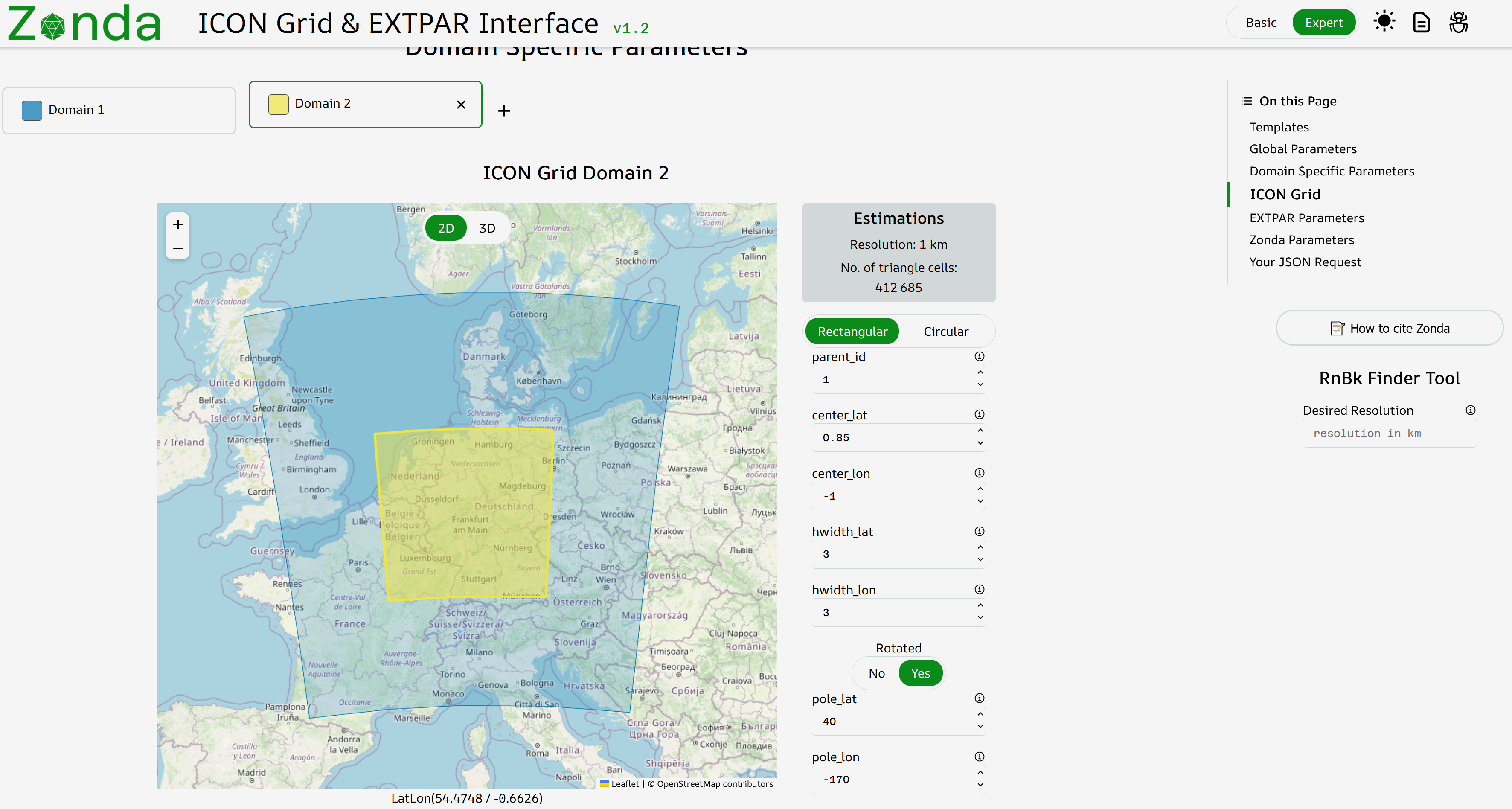
Zonda is a web interface designed to facilitate the generation of ICON grid files and External Parameter data (ExtPar) on ICON triangular grids for research and on-demand simulations. Zonda makes use of containerized versions of the ICON grid generator and ExtPar. It constructs the Fortran and Python namelist setups and runs the containers on a public server.
The invocation of Zonda is realized as a two-step process:
In the frontend (see the Zonda website for details), the user specifies the domain(s) including the appropriate settings for the external parameter generation. Example configurations and an expert mode with additional choices are available to assist the user. The user gets a
JSONcode snippet containing the chosen configuration which is required for the second step.In the backend (see Zonda Request for details), the JSON code has to be pasted into a Github issue. Then, the Github CI triggers the generation of the ICON Grid and ExtPar data. These files in
NetCDF 4format are then provided as.zipfile.
The Zonda web interface comes with Documentation. Furthermore, the available options in the frontend contain tooltips with short descriptions and links to the documentation of the respective option.
Congratulations! You have successfully completed Exercise 3.
Further Reading and Resources#
Necessary Input Data
ICON Manual, Ch. 2: https://www.dwd.de/DE/leistungen/nwv_icon_tutorial/nwv_icon_tutorial.html
A new draft version of the ICON Tutorial is available here: https://icon-training-2025-scripts-rendering-cc74a6.gitlab-pages.dkrz.de/index.html. It is currently being finalized and will be published soon.GRIB parameter database (ECMWF): https://apps.ecmwf.int/codes/grib/param-db/
Data supply
Automatic File Distribution (AFD) service: https://www.dwd.de/EN/aboutus/it/functions/Teasergroup/applications.html?nn=24864#AFD
Zonda Grid and ExtPar web interface:
Website: https://zonda.ethz.ch/
Documentation: https://zonda.ethz.ch/docs
Zonda Request: https://github.com/C2SM/zonda-request
Public list of ICON grids: http://icon-downloads.mpimet.mpg.de/dwd_grids.xml
Author info: Deutscher Wetterdienst (DWD) 2025 :: icon@dwd.de. For a full list of contributors, see CONTRIBUTING in the root directory. License info: see LICENSE file.