
ICON Training - Hands-on Session
Exercise 5: Programming ICON#
|
In this step-by-step exercise we will learn how to implement new variables in the ICON source code. In the first and relatively easy part of the exercise we will modify the Fortran code directly:
|
|
Step F1: Allocating Additional Fields in the Fortran Code#
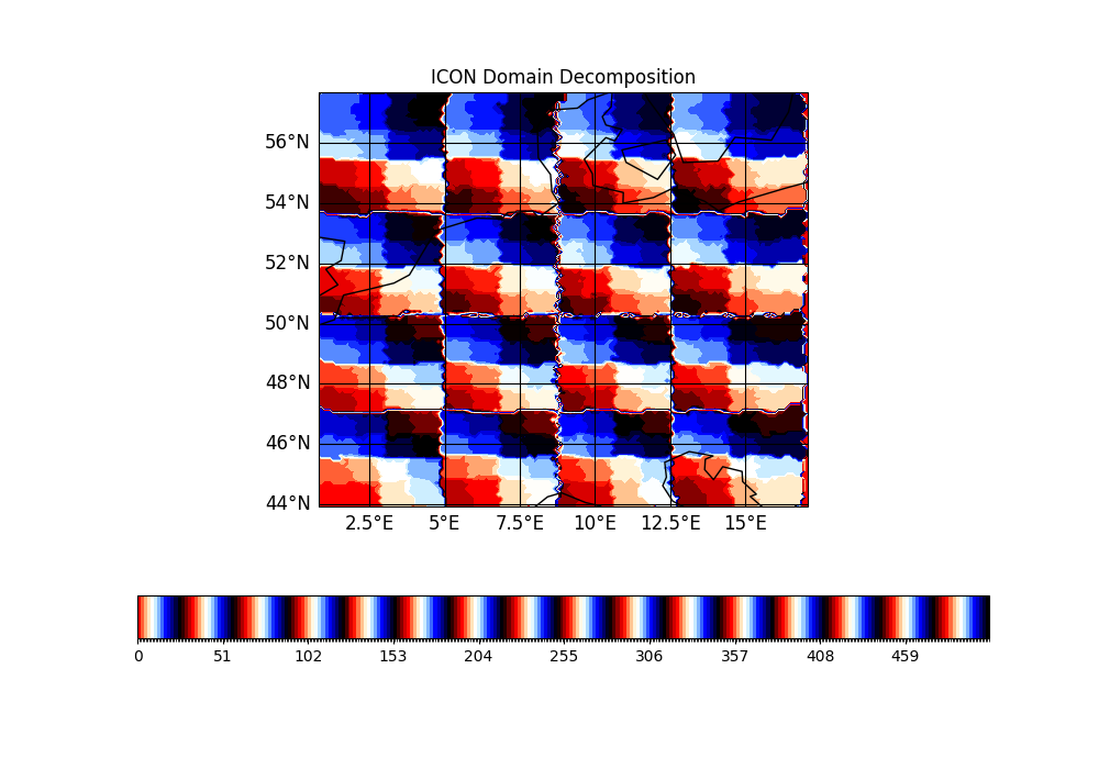
In the following we will allocate a new ICON variable directly in the Fortran code. As a by-product we will visualize ICON’s domain decomposition.
Details are given in Section 9.4 of the ICON Tutorial (see the link at the bottom of the page).
/scratch/${USER::1}/$USER/icon. To this end, follow these steps closely:
 export SCRATCHDIR=/scratch/${USER::1}/$USER
 export ICONDIR=${SCRATCHDIR}/icon
Download the release ICON-2025.04-1 as follows:
( cd ${SCRATCHDIR}
  git clone --recursive --branch release-2025.04-public https://gitlab.dkrz.de/icon/icon-model.git icon )
cython, a tool that allows us to create interfaces between C or C++ and Python. We also modify the wrapper script with an additional linker flag:
Adding -Wl,--export-dynamic-symbol=yac_* to both the host model and plugin linking flags ensures YAC is only loaded once, preventing duplicate copies of its internal lookup table.
cd $ICONDIR
pip install cython

sed -i 's|LDFLAGS="${LDFLAGS}"|LDFLAGS="${LDFLAGS} -Wl,--export-dynamic"|' config/dkrz/levante.gcc-11.2.0
We then execute the configure wrapper for the ‘Levante’ platform with the GCC compiler (config/dkrz/levante.gcc) in our local copy of the ICON code.
These steps are fully documented in the ICON Quickstart Guide.
We set several options:
--enable-comin
Enables the use of the ICON Community Interface (ComIn), a plugin mechanism which will be used in later exercises.--enable-bundled-python
enables the Python interfaces for ComIn.--disable-jsbach
Disables the JSBACH land surface model, which simulates land biosphere processes such as vegetation, soil, carbon, and water cycles.--disable-quincy
Disables the QUINCY land surface model, an alternative model for land surface biogeochemistry and vegetation.--disable-rte-rrtmgp
Disables the RTE+RRTMGP radiation scheme, an advanced radiative transfer model for calculating radiative fluxes and heating rates in the atmosphere.
mkdir -p $ICONDIR/build
cd $ICONDIR/build

../config/dkrz/levante.gcc \
  --enable-comin --disable-jsbach --disable-quincy --disable-rte-rrtmgp --enable-bundled-python  --disable-silent-rules \
> configure.log
Now the ICON code is ready and can be compiled with make in the following exercise.
Perform the following changes step-by-step:#
Just to ensure that our experiment directory is in the correct location:
export SCRATCHDIR=/scratch/${USER::1}/$USER
In the subdirectory
src/atm_dyn_iconamopen the modulemo_nonhydro_types.
This file contains important structure declarations, i.e. the names and characteristics of the data objects in the atmospheric model:Insert a new 2D variable pointer
process_idof typeREAL(wp)to the derived typeTYPE(t_nh_diag).
Open the module
mo_nonhydro_statein the same subdirectory.
This file allocates the storage for the above data objects.At the end of the subroutine
new_nh_state_diag_listset appropriate metadata variables for NetCDF.
(
standard_name,units,long_name,datatype; seet_cf_var)set the metadata also for GRIB2.
(You may use dummy numbers:
discipline = parameterCategory = parameterNumber = 255)place the
add_varcall for the new field.
Now, after the
add_varcall, the new field has been allocated. Fill the data array with a constant value:process_id(:,:) = get_my_mpi_work_id()This auxiliary function from the source code module
mo_mpireturns the MPI rank of the processor (see Section 9.2.4 of the ICON tutorial).
Solution
(Search for EX5:ProgrammingICON:AllocatingFields)
Build Process#
build directory, where we have executed the configure wrapper for the "Levante" platform with the gcc compiler (config/dkrz/levante.gcc, see above).
Execute make with 4 processes.
Due to the large amount of log output during the configuration and compiling, we highly recommend performing this exercise in a terminal window.
export ICONDIR=$SCRATCHDIR/icon

...
Solution
export SCRATCHDIR=/scratch/${USER::1}/$USER
export ICONDIR=$SCRATCHDIR/icon
cd $ICONDIR/build

make -j4 2>&1 > compile.log
Run the ICON model & visualize the results#
|
|
Solution
Each PE writes a different (constant) value - its MPI rank.
Solution
This is a lat-lon interpolated field; although the original field has only integer values, we get intermediate values in the lat-lon interpolation.
Optional Exercise: Looping over grid points in Fortran#
process_id to the MPI rank of the processor only for prognostic cells. For all other cells, set process_id to -1. To achieve this, you must write loops that iterate over the prognostic cells.
Explanation of looping in ICON
For more detailed information, refer to Section 9.3 of the ICON tutorial (see the link at the bottom of the page).
In order to enhance computational efficiency, loops that iterate over grid cells, edges, and vertices are structured using nested loops, which are known as
jbloops andjcloops. The jb loop is typically employed as the outer loop and is often parallelized using OpenMP.This approach involves breaking down a long vector into smaller chunks of length
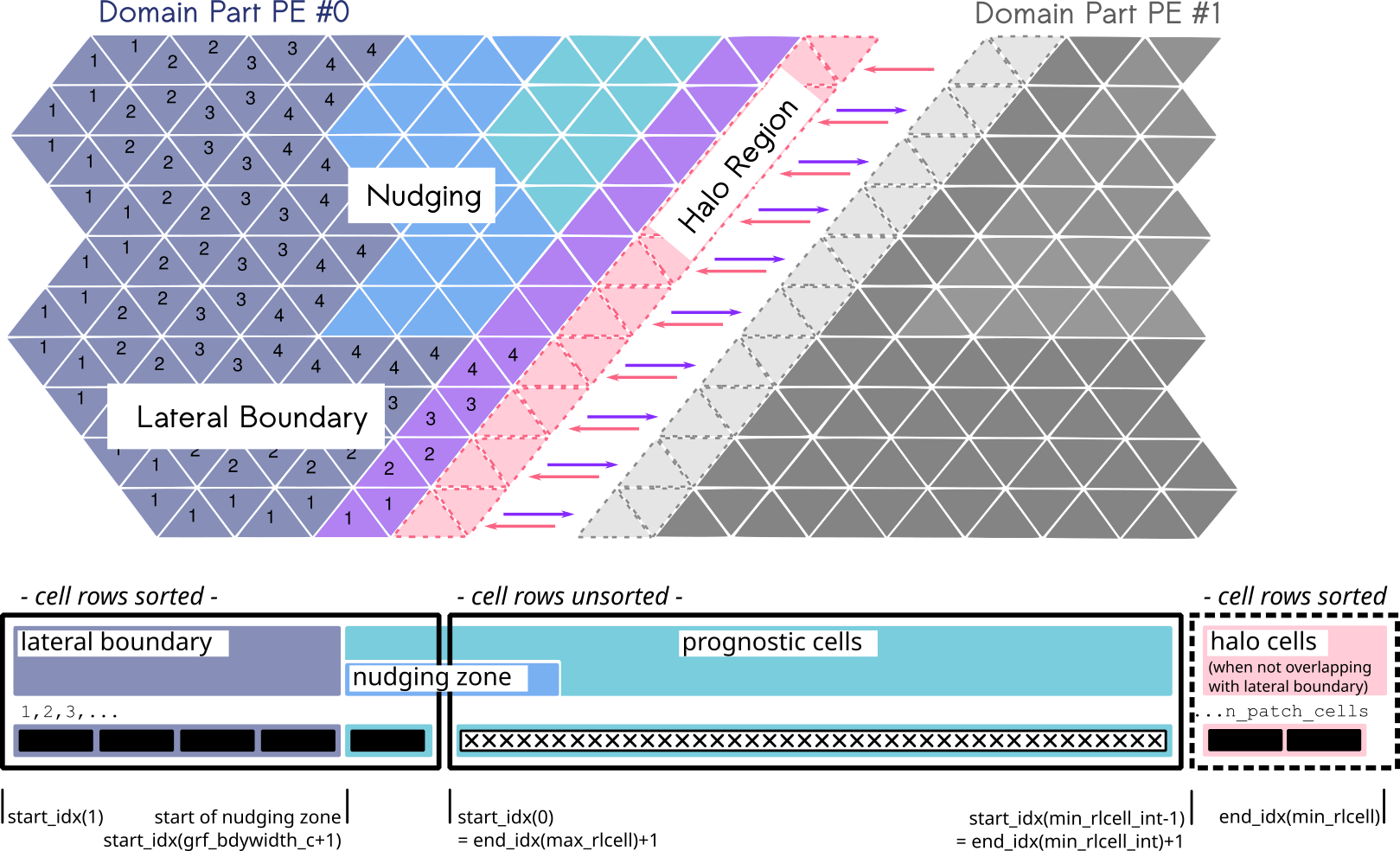
nproma. The long vector is stored in a two-dimensional array, where the first index represents the number of elements within a block (jc), and the second index represents the number of blocks (jb).Upon examination of the figure above (Figure 9.2 in the ICON tutorial), it becomes apparent that by selecting the
start_idx(start index for looping over the blocks) andend_idx(end index for looping over the blocks), one can determine which cell types (boundary regions, prognostic cells, or halo cells) to include in the loop.In the event that
npromadoes not divide the number of cells evenly, the final block may not be completely filled. It therefore is necessary that for each block (jb), the start and end indices of the elements within the block are calculated. The auxiliary functionget_indices_cin ICON assists in computing these indices.
Hints:
Open the module
mo_nh_stepping(subdirectorysrc/atm_dyn_iconam).Create an (empty) subroutine.
Place a call to this subroutine immediately before the call to the output routine in the timeloop.
Fill your subroutine with a 2D loop over all prognostic grid points, see p. 205 of the ICON tutorial (see the link at the bottom of the page) for help.
Solution
(Search for EX5:ProgrammingICON:LoopOverGridPoints)
Congratulations! You have successfully completed Exercise 5.
Further Reading and Resources#
ICON Tutorial, Ch. 9: https://www.dwd.de/DE/leistungen/nwv_icon_tutorial/nwv_icon_tutorial.html
A new draft version of the ICON Tutorial is available here: https://icon-training-2025-scripts-rendering-cc74a6.gitlab-pages.dkrz.de/index.html. It is currently being finalized and will be published soon.
Author info: Deutscher Wetterdienst (DWD) 2025 :: icon@dwd.de. For a full list of contributors, see CONTRIBUTING in the root directory. License info: see LICENSE file.