
ICON Training - Hands-on Session
Exercise 2: Global Real Data Run#
The course exercises revisit the topics of the individual tutorial chapters and range from easy tests to the setup of complex forecast simulations.
In this particular exercise you will learn how to
start a global ICON forecast from DWD analysis data
activate a nest over Europe
configure the ICON model output namelist
example: creating boundary data for driving a limited area ICON
make use of the ICON LOG output
Note: This script is not suited for operational use, it is part of the step-by-step tutorial. Furthermore, we will omit some of ICON’s less important input and output channels here, e.g. the restart files. This exercise focuses on command-line tools and the rudimentary visualization with Python scripts. Professional post-processing and viz tools are beyond the scope of this tutorial.
Input Data#
Global ICON-NWP runs require a number of input data, in particular
- grid files: coordinates and topological index relations between cells, edges and vertices
- external parameter files: time invariant fields such as topography, lake depths or soil type
- initial conditions: snapshot of an atmospheric state and soil state from which the model is integrated forward in time
This data is already available in the directory /pool/data/ICON/ICON_training/exercise_realdata.
On default, ICON expects the input data to be located in the experiment directory (termed $EXPDIR in the run scripts).
The run script creates symbolic links in the experiment directory, which point to the input files.
Setup#
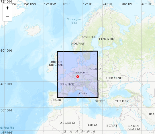
We prepare a global forecast with 40 km horizontal grid spacing and a 20 km nest over Europe. More details are given in the table below.
Configuration |
global |
nest |
|---|---|---|
mesh size |
40 km (R2B6) |
20 km (R2B7) |
model top height |
75 km |
23 km |
no. of levels |
90 |
60 |
no. of cells (per level) |
327680 |
9376 |
time step |
360 s |
180 s |
duration |
48h |
(see exercise) |
# base directory for ICON sources and binary:
ICONDIR=/pool/data/ICON/ICON_training/icon/

# directory with input grids and external data:
GRIDDIR=/pool/data/ICON/ICON_training/exercise_realdata/grids
# directory with initial data:
DATADIR=/pool/data/ICON/ICON_training/exercise_realdata/data/ini

# absolute path to directory with plenty of space:
SCRATCHDIR=/scratch/${USER::1}/$USER
EXPDIR=$SCRATCHDIR/exercise_realdata

# absolute path to files needed for radiation
RADDIR=${ICONDIR}/externals/ecrad/data

# path to prepared namelists
NMLDIR=$HOME/icon-training-scripts/exercise_realdata/nml
$EXPDIR: grids, external parameters, initial conditions.
The directory for the experiment will be created, if not already there.
if [ ! -d $EXPDIR ]; then
    mkdir -p $EXPDIR
fi
cd ${EXPDIR}

# grid files: link to output directory
ln -sf ${GRIDDIR}/iconR*.nc .
# external parameter files: link to output directory
ln -sf ${GRIDDIR}/extpar*.nc .
# analysis files: link to output directory
ln -sf ${DATADIR}/*.grb .

# Dictionary for the mapping: DWD GRIB2 names <-> ICON internal names
ln -sf ${ICONDIR}/run/ana_varnames_map_file.txt map_file.ana

# For Output: Dictionary for the mapping: names specified in the output nml <-> ICON internal names
ln -sf ${ICONDIR}/run/dict.output.dwd dict.output.dwd
$EXPDIR by using, for example, the ls linux command.
Solution
lrwxrwxrwx 1 m300173 mh0287    55 Jul  7 14:52 dict.output.dwd -> /pool/data/ICON/ICON_training/icon//run/dict.output.dwd
lrwxrwxrwx 1 m300173 mh0287    79 Jul  7 14:52 dwdANA_R2B06_DOM01.grb -> /pool/data/ICON/ICON_training/exercise_realdata/data/ini/dwdANA_R2B06_DOM01.grb
lrwxrwxrwx 1 m300173 mh0287    79 Jul  7 14:52 dwdANA_R2B07_DOM02.grb -> /pool/data/ICON/ICON_training/exercise_realdata/data/ini/dwdANA_R2B07_DOM02.grb
lrwxrwxrwx 1 m300173 mh0287    69 Jul  7 14:52 extpar_DOM01.nc -> /pool/data/ICON/ICON_training/exercise_realdata/grids/extpar_DOM01.nc
lrwxrwxrwx 1 m300173 mh0287    69 Jul  7 14:52 extpar_DOM02.nc -> /pool/data/ICON/ICON_training/exercise_realdata/grids/extpar_DOM02.nc
lrwxrwxrwx 1 m300173 mh0287    72 Jul  7 14:52 iconR2B05_DOM00.nc -> /pool/data/ICON/ICON_training/exercise_realdata/grids/iconR2B05_DOM00.nc
lrwxrwxrwx 1 m300173 mh0287    72 Jul  7 14:52 iconR2B06_DOM01.nc -> /pool/data/ICON/ICON_training/exercise_realdata/grids/iconR2B06_DOM01.nc
lrwxrwxrwx 1 m300173 mh0287    72 Jul  7 14:52 iconR2B07_DOM02.nc -> /pool/data/ICON/ICON_training/exercise_realdata/grids/iconR2B07_DOM02.nc
lrwxrwxrwx 1 m300173 mh0287    65 Jul  7 14:52 map_file.ana -> /pool/data/ICON/ICON_training/icon//run/ana_varnames_map_file.txt
#
Prepare the ICON run (namelists etc.)#
Create the ICON master namelist#
The start date is
2021-07-13T00:00:00
i.e. July 13, 2021.
The forecast time is
48 hours
ini_datetime_string and end_datetime_string. See Section 5.1.1 of the
ICON tutorial "Basic Settings for Running Real Data Runs" for details .
cat > icon_master.namelist << EOF

! master_nml: ----------------------------------------------------------------
&master_nml
 lrestart                   =                      .FALSE.        ! .TRUE.=current experiment is resumed
/

! master_model_nml: repeated for each model ----------------------------------
&master_model_nml
 model_type                  =                          1         ! identifies which component to run (atmosphere,ocean,...)
 model_name                  =                       "ATM"        ! character string for naming this component.
 model_namelist_filename     =              "NAMELIST_NWP"        ! file name containing the model namelists
 model_min_rank              =                          1         ! start MPI rank for this model
 model_max_rank              =                      65536         ! end MPI rank for this model
 model_inc_rank              =                          1         ! stride of MPI ranks
/

! time_nml: specification of date and time------------------------------------
&time_nml
 ini_datetime_string         =      "??????????????"        ! initial date and time of the simulation
 end_datetime_string         =      "??????????????"        ! end date and time of the simulation
                                                            ! example date: 2001-01-01T01:00:00Z
 dt_restart                  =      1000000.
/

EOF
Solution
&time_nml
ini_datetime_string         =      "2021-07-13T00:00:00Z"  ! initial date and time of the simulation
end_datetime_string         =      "2021-07-15T00:00:00Z"  ! end date and time of the simulation
#
Create the ICON model namelists#
In the following we will build up the ICON namelist NAMELIST_NWP step by step. To do so, we use the UNIX cat command in order to collect individual namelists into a single file (named NAMELIST_NWP).
for a complete list of Namelist parameters see Namelist_overview.pdf
Please make sure that you execute each of the following cells only once!
Due to the command cat >> NAMELIST_NWP << EOF (note the double >>), the namelist groups such as parallel_nml below will be concatenated each time you execute the cell.
- Set the namelist parameters
ltestcase,ldynamics,ltransport, andiforcingfor a real data NWP run. See Section 5.1.1 ("Basic Settings for Running Real Data Runs") of the tutorial for details.
- Activate a global R2B6 domain with R2B7 nest by specifying the list of horizontal grids to be used (
dynamics_grid_filename). See Section 4.1.2, "Specifying the Computational Domain(s)", of the tutorial. - In order to save computational resources, the nested domain should have a reduced model top height and comprise only the lowermost 60 vertical levels of the global domain (instead of 90 levels). Please specify
num_lev(run_nml) accordingly. See Section 4.1.2, "Specifying the Computational Domain(s)", of the tutorial. - Specify the grid on which radiation will be computed
radiation_grid_filename. Radiation should be computed on a coarser (reduced) grid with half the resolution for both domains. See Section 3.10, "Reduced Radiation Grid", of the tutorial.
lredgrid_phys=.TRUE.,.TRUE., which has already been prepared for you.
cat > NAMELIST_NWP << EOF

! run_nml: general switches ---------------------------------------------------
&run_nml
 ltestcase                   =              ?????????????         ! idealized testcase runs
 num_lev                     =              ?????????????         ! number of full levels (atm.) for each domain
 lvert_nest                  =                      .TRUE.        ! vertical nesting
 dtime                       =                        360.        ! timestep in seconds
 ldynamics                   =              ?????????????         ! compute adiabatic dynamic tendencies
 ltransport                  =              ?????????????         ! compute large-scale tracer transport
 ntracer                     =                          5         ! number of advected tracers
 iforcing                    =              ?????????????         ! forcing of dynamics and transport by parameterized processes
                                                                  ! 2: AES physics package
                                                                  ! 3: NWP physics package
 msg_level                   =                         13         ! controls how much printout is written during runtime
 ltimer                      =                      .FALSE.       ! timer for monitoring the runtime of specific routines
 timers_level                =                          1         ! performance timer granularity
 output                      =                       "nml"        ! main switch for enabling/disabling components of the model output
/

! grid_nml: horizontal grid --------------------------------------------------
&grid_nml
 dynamics_grid_filename      =                 ??????????         ! array of the grid filenames for the dycore
 radiation_grid_filename     =                 ??????????         ! grid filename for the radiation model
 lredgrid_phys               =               .TRUE.,.TRUE.        ! .true.=radiation is calculated on a reduced grid
 lfeedback                   =                      .TRUE.        ! specifies if feedback to parent grid is performed
 ifeedback_type              =                          2         ! feedback type (incremental/relaxation-based)
 start_time                  =                     0.,  0.        ! Time when a nested domain starts to be active [s]
 end_time                    =                  0., 86400.        ! Time when a nested domain terminates [s]
 nexlevs_rrg_vnest           =                         14         ! numer of extra model layers for radiation
/

EOF
Solution
&run_nml
 ltestcase                   =                    .FALSE.         ! idealized testcase runs
 num_lev                     =                     90,60          ! number of full levels (atm.) for each domain
 ldynamics                   =                     .TRUE.         ! compute adiabatic dynamic tendencies
 ltransport                  =                     .TRUE.         ! compute large-scale tracer transport
 iforcing                    =                          3         ! forcing of dynamics and transport by parameterized processes

&grid_nml
 dynamics_grid_filename      = 'iconR2B06_DOM01.nc','iconR2B07_DOM02.nc' ! array of the grid filenames for the dycore
 radiation_grid_filename     =       'iconR2B05_DOM00.nc'         ! grid filename for the radiation model
- For improved runtime performance, activate asynchronous output by setting the number of dedicated I/O processors (
num_io_procs) to a value larger than 0 (e.g. 2). See Section 8.2 ("Settings for Parallel Execution") of the tutorial for more details on the asynchronous output module.
cat >> NAMELIST_NWP << EOF
! parallel_nml: MPI parallelization -------------------------------------------
¶llel_nml
nproma = 32 ! loop chunk length
p_test_run = .FALSE. ! .TRUE. means verification run for MPI parallelization
num_io_procs = ????????????? ! number of I/O processors
num_restart_procs = 0 ! number of restart processors
iorder_sendrecv = 3 ! sequence of MPI send/receive calls
num_dist_array_replicas = 10 ! distributed arrays: no. of replications
use_omp_input = .TRUE. ! allows task parallelism for reading atmospheric input data
/
EOF
Solution
¶llel_nml
num_io_procs = 2 ! number of I/O processors
#
- Set the appropriate
itopovalue for real data runs and specify the name of the external parameter file (extpar_filename). Rather than specifying a comma-separated list of filenames, you must make use of the keyword<idom>. See Section 5.1.1 of the tutorial ("Basic Settings for Running Real Data Runs") for more details on keywords.
$EXPDIR.
cat >> NAMELIST_NWP << EOF

! extpar_nml: external data --------------------------------------------------
&extpar_nml
 itopo                       =              ?????????????         ! topography (0:analytical)
 itype_lwemiss               =                          2         ! requires updated extpar data
 itype_vegetation_cycle      =                          1         ! specifics for annual cycle of LAI
 extpar_filename             =              ?????????????         ! filename of external parameter input file
 n_iter_smooth_topo          =                        1,1         ! iterations of topography smoother
 hgtdiff_max_smooth_topo     =                   750.,750.        ! see Namelist doc
 pp_sso                      =                          1         ! type of postprocessing for SSO standard deviation
 read_nc_via_cdi             =                      .TRUE.        ! TRUE/FALSE: read NetCDF input data using CDI or parallel NetCDF library
/

EOF
Solution
&extpar_nml
itopo                       =                          1         ! topography (0:analytical)
extpar_filename             =       'extpar_DOM<idom>.nc'        ! filename of external parameter input file
#
- The model shall be started from an initialized DWD analysis. Set the appropriate initialization mode
init_mode. See Tutorial Section 5.1.4, "Starting from Initialized DWD Analysis". - Specify the name (and path) of the initial data (analysis) file by setting the Namelist parameter
dwdfg_filename - Instead of specifying the full name, make use of the keywords
<nroot>,<jlev>,<idom>. See Section 5.1.2 of the tutorial for a list of available keywords. - Hint: Identify the initial data file (analysis) in your current working directory
$EXPDIR. You can make use of relative or absolute paths. - Activate surface tiles.
Please activate 3 dominant land tiles per grid cell by setting
ntiles(lnd_nml) appropriately. Since the initial data contain aggregated (cell averaged) surface fields, a tile coldstart must be performed, i.e. each surface tile must be initialized with the same cell averaged value. The corresponding namelist switch is termedltile_coldstart(see Section 3.8.9, "Land-Soil Model TERRA").
cat >> NAMELIST_NWP << EOF

! initicon_nml: specify read-in of initial state ------------------------------
&initicon_nml
 init_mode                  =              ?????????????         ! start from initialized DWD analysis
 dwdfg_filename             =              ?????????????         ! initialized analysis data
 ltile_coldstart            =              ?????????????         ! coldstart for surface tiles
 lp2cintp_sfcana            =                       .TRUE.       ! interpolate surface analysis from global domain onto nest
 ana_varnames_map_file      =                'map_file.ana'      ! dictionary mapping internal names onto GRIB2 shortNames
/
! lnd_nml: land scheme switches -----------------------------------------------
&lnd_nml
 ntiles                      =              ?????????????         ! number of land tiles
 nlev_snow                   =                          3         ! number of snow layers
 lmulti_snow                 =                      .FALSE.       ! .TRUE. for use of multi-layer snow model
 idiag_snowfrac              =                         20         ! type of snow-fraction diagnosis
 lsnowtile                   =                       .TRUE.       ! .TRUE.=consider snow-covered and snow-free separately
 itype_canopy                =                          2         ! Type of canopy parameterization
 itype_root                  =                          2         ! root density distribution
 itype_trvg                  =                          3         ! BATS scheme with add. prog. var. for integrated plant transpiration since sunrise
 itype_evsl                  =                          4         ! type of bare soil evaporation
 itype_heatcond              =                          3         ! type of soil heat conductivity
 itype_lndtbl                =                          4         ! table for associating surface parameters
 itype_snowevap              =                          3         ! Snow evap. in vegetated areas with add. variables for snow age and max. snow height
 cwimax_ml                   =                          5.e-4     ! scaling parameter for maximum interception parameterization
 c_soil                      =                          1.25      ! surface area density of the (evaporative) soil surface
 c_soil_urb                  =                          0.5       ! surface area density of the (evaporative) soil surface, urban areas
 lseaice                     =                      .TRUE.        ! .TRUE. for use of sea-ice model
 llake                       =                      .TRUE.        ! .TRUE. for use of lake model
 lprog_albsi                 =                      .TRUE.        ! sea-ice albedo is computed prognostically
 sstice_mode                 =                          2         ! SST is updated by climatological increments on a daily basis
/

EOF
Solution
&initicon_nml
init_mode                  =                          7                ! start from initialized DWD analysis
dwdfg_filename             ='./dwdANA_R<nroot>B<jlev>_DOM<idom>.grb'   ! initialized analysis data
ltile_coldstart            =                       .TRUE.              ! coldstart for surface tiles

&lnd_nml
ntiles                     =                           3               ! number of tiles
#
$NMLDIR/NAMELIST_NWP_base, by executing the following cell.
cat $NMLDIR/NAMELIST_NWP_base >> NAMELIST_NWP
#
The initial conditions file (i.e. here the initialized analysis) is provided via the namelist parameter dwdfg_filename (initicon_nml), see Section 5.1.4 “Starting from Initialized DWD Analysis”, of the tutorial.
As an exercise you have been asked to set the file name, using the keyword nomenclature.
In the following small exercise, we will try to understand how these keywords work.
dwdfg_filename = './dwdANA_R<nroot>B<jlev>_DOM<idom>.grb'?
dwdANA_R3B06.grbdwdANA_R2B6_DOM01.grbdwdANA_R9B02_DOM02.grbdwdana_R2B06_DOM01.grb
Solution
[ ]
dwdANA_R3B06.grb: no, “DOM…” missing[ ]
dwdANA_R2B6_DOM01.grb: no, only single digit[x]
dwdANA_R9B02_DOM02.grb: yes[ ]
dwdana_R2B06_DOM01.grb: no on case-sensitive Linux file system
#
|
Exercise (One-way versus two-way nesting):
Open a terminal and navigate to the experiment directory EXPDIR, where you will find the full model namelist NAMELIST_NWP.Have a look at the namelist group grid_nml, to find out about the following nesting details.
|
|
Answer: One-way versus two-way nesting
Answer: Nested domain start and end times
Solution
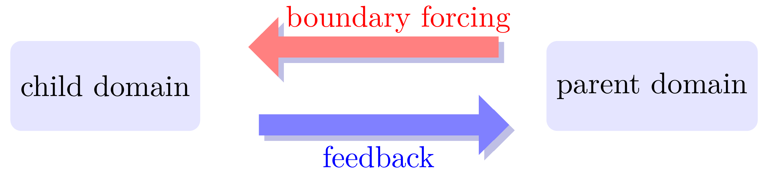
The domain over Europe is two-way nested. (Incremental) feedback to the global domain is turned on.
&grid_nml
 lfeedback                   =                      .TRUE.        ! specifies if feedback to parent grid is performed
The nested domain starts at 2021-07-13T00:00:00 (model start) and terminates after one day at 2021-07-14T00:00:00.
&grid_nml
 start_time                  =                    0.,  0.        ! Time when a nested domain starts to be active [s]
 end_time                    =                 0., 86400.        ! Time when a nested domain terminates [s]
#
Running the model and inspecting the output#
Execute the following cell, in order to create the ICON batch job file (job will not be submitted to the HPC cluster)
cat > $EXPDIR/icon.sbatch << 'EOF'
#!/bin/bash
#SBATCH --job-name=testjob
#SBATCH --partition=compute
#SBATCH --nodes=6
#SBATCH --ntasks-per-node=128
#SBATCH --output=slurm.%j.out
#SBATCH --exclusive
#SBATCH --mem-per-cpu=960
#SBATCH --time=00:20:00

### ENV ###
env
set -xe

unset SLURM_EXPORT_ENV
unset SLURM_MEM_PER_NODE
unset SBATCH_EXPORT

ulimit -c 0 # limit core file size
ulimit -l unlimited

export SLURM_DIST_PLANESIZE="32"
export OMPI_MCA_btl="self"
export OMPI_MCA_coll="^ml,hcoll"
export OMPI_MCA_io="romio321"
export OMPI_MCA_osc="ucx"
export OMPI_MCA_pml="ucx"
export UCX_HANDLE_ERRORS="bt"
export UCX_TLS="shm,dc_mlx5,dc_x,self"
export UCX_UNIFIED_MODE="y"
export MALLOC_TRIM_THRESHOLD_="-1"
export OMPI_MCA_pml_ucx_opal_mem_hooks=1

module load eccodes

export ECCODES_DEFINITION_PATH=/pool/data/ICON/ICON_training/eccodes/definitions.edzw-2.27.0-1:$ECCODES_DEFINITION_PATH
export OMP_NUM_THREADS=1

# path to model binary, including the executable:
MODEL=$ICONDIR/build/bin/icon

srun -l --cpu_bind=verbose --hint=nomultithread --distribution=block:cyclic $MODEL

EOF
Running the ICON model#
Submit the job to the HPC cluster, using the Slurm command sbatch.
export ICONDIR=$ICONDIR
cd $EXPDIR && sbatch --account=$SLURM_JOB_ACCOUNT icon.sbatch
Checking the job status#
Check the job status via squeue.
Inspecting the Model Output#
After the job has finished, inspect the model output. Take a look at the output files in $EXPDIR.
How can you identify which file is which (apart from the obvious file names that we have chosen)? Use
cdo sinfov to identify the relevant metadata.
Hint: You might have to load the environment modules cdo
Answer: native
Answer: lat/lon
Solution
Answer: native
output on native grid : NWP_DOM01_ML_0001.nc (grid coordinates = ‘unstructured’)
Answer: lat/lon
output on lat/lon grid: NWP_lonlat_DOM01_ML_0001.nc (grid coordinates = ‘lonlat’)
cd $EXPDIR
module load cdo

set +o xtrace
cdo sinfov NWP_DOM01_ML_0001.nc  | grep  -B0 -A1 "Grid coordinates"
cdo sinfov NWP_lonlat_DOM01_ML_0001.nc  | grep  -B0 -A1 "Grid coordinates"
#
cdo sinfov to identify the type of atmospheric vertical output grid.
- model level (ML)
- pressure level (PL)
- height level (HL)
Solution
SAMPLE SOLUTION: Type of atm. vertical output grid : ML = “model levels” (CDO depicts generalized_height)
cd $EXPDIR
module load cdo
cdo sinfov NWP_lonlat_DOM01_ML_0001.nc | grep "Vertical coordinates" -B0 -A1
#
ncview for visualizing the interpolated lat-lon output.
#
Time-stepping#
|
This exercise focuses on aspects of the ICON time-stepping scheme, explained in Section 3.7.1, "ICON Time-Stepping". |

|
Compute the dynamics time step Δτ from the specification of the physics time step Δt (
dtime) and the number of dynamics substeps ndyn_substeps (nonhydrostatic_nml).
Hint: Have a look at the model Namelist
$EXPDIR/NAMELIST_NWP
Solution
Answer: 360s/5 = 72s
#
The timestep is proportional to the effective mesh size \(\overline{\Delta x}\) of the horizontal ICON grid.
Compare this to the time step used: Did we make a reasonable choice?
Solution
Answer: The effective mesh size of a global grid can be estimated as
\( \overline{\Delta x} \approx 5050/(n\,2^k) \quad [\mathrm{km}]\,. \)
Example Python code
python3 - << EOF
n = 2 # grid_root
k = 6 # grid_level

mesh_size = 5050/(n * 2**k) # [km]
print(f"mesh size: {mesh_size} [km]")

delta_tau_max = 1.8 * mesh_size
print(f"delta tau_max: {delta_tau_max} [s]");
EOF
Result
\(\Delta \tau_{max} = 1.8 \cdot 10^{-3} \cdot 39453.125 ~[s] \approx 71 ~[s] \)
#
Optional: Appending your own output namelist#
Forcing data should be written
- in GRIB2 format
- for the EU-nest only
- 2-hourly, beginning at model start until 24 hours forecast time
- with one output step per file
- on the native (triangular) grid
- into the subdirectory `lam_forcing` of your output directory, using the filename prefix `forcing`. If the subdirectory does not exist, please create.
- containing model level output for
U,V,W,PRES,TEMP,QV,QC,QI,QR,QS,HHL.
cat >> NAMELIST_NWP << EOF

!----------------------------------------------------------------------------
! output_nml: writing boundary data for LAM                             ;----
!----------------------------------------------------------------------------
&output_nml
 filetype                    =              ?????????????         ! output format: GRIB2 or NETCDFv2
 dom                         =              ?????????????         ! write output only for EU-nest
 output_bounds               =              ?????????????         ! output: start, end, increment in s
 steps_per_file              =              ?????????????         ! number of output steps in one output file
 remap                       =              ?????????????         ! (no)remap to regular lat/lon grid (0 or 1)
 output_grid                 =                     .FALSE.        ! flag whether grid information is added to output.
 output_filename             =              ?????????????         ! file name base
 filename_format             = '<output_filename>_<levtype>_<datetime2>' ! full file format
 mode                        =                          1         ! 1: forecast mode (relative t-axis), 2: climate mode (absolute t-axis)
 !
 ml_varlist                  =              ?????????????         ! output fields on model levels
/

EOF
Solution
cat >> NAMELIST_NWP << EOF

!----------------------------------------------------------------------------
! output_nml: LAM exercise;  writing boundary data for LAM              ;----
!----------------------------------------------------------------------------
&output_nml
 filetype                    =                          2         ! output format: GRIB2 or NETCDFv2
 dom                         =                          2         ! write output only for EU-nest
 output_bounds               =          0., 86400., 7200.         ! output: start, end, increment in s
 steps_per_file              =                          1         ! number of output steps in one output file
 remap                       =                          0         ! (no)remap to regular lat/lon grid (0 or 1)
 output_grid                 =                     .FALSE.        ! flag whether grid information is added to output.
 output_filename             =     './lam_forcing/forcing'        ! file name base
 filename_format             = '<output_filename>_<levtype>_<datetime2>' ! full file format
 mode                        =                          1         ! 1: forecast mode (relative t-axis), 2: climate mode (absolute t-axis)
 !
 ml_varlist                  = 'U','V','W','PRES','TEMP','QV','QC','QI','QR','QS','HHL'  ! output fields on model levels
/

EOF
#
Then, create the additional output directory:
mkdir -p $EXPDIR/lam_forcing
Submit the batch job.
export ICONDIR=$ICONDIR
cd $EXPDIR && sbatch --account=$SLURM_JOB_ACCOUNT icon.sbatch
Check the job status via squeue.
#
Check the correctness of your output files. You should find 13 forcing data files in your output directory lam_forcing.
export ECCODES_DEFINITION_PATH=/pool/data/ICON/ICON_training/eccodes/definitions.edzw-2.27.0-1:$ECCODES_DEFINITION_PATH
cdo sinfov data-file.grb > data-file.sinfov
   File format : GRIB2
    -1 : Institut Source   T Steptype Levels Num    Points Num Dtype : Parameter name
     1 : DWD      unknown  v instant      60   1      9376   1  P16  : U
     2 : DWD      unknown  v instant      60   1      9376   1  P16  : V
     3 : DWD      unknown  v instant      61   2      9376   1  P16  : W
     4 : DWD      unknown  v instant      60   1      9376   1  P16  : P
     5 : DWD      unknown  v instant      60   1      9376   1  P16  : T
     6 : DWD      unknown  v instant      60   1      9376   1  P16  : QV
     7 : DWD      unknown  v instant      60   1      9376   1  P16  : QC
     8 : DWD      unknown  v instant      60   1      9376   1  P16  : QI
     9 : DWD      unknown  v instant      60   1      9376   1  P16  : QR
    10 : DWD      unknown  v instant      60   1      9376   1  P16  : QS
    11 : DWD      unknown  v instant      61   3      9376   1  P16  : HHL
   Grid coordinates :
     1 : unstructured             : points=9376
                             grid : number=101  position=1
                             uuid : 7f1e5eb3-fc61-a692-b99f-830dab7e2440
   Vertical coordinates :
     1 : generalized_height       : levels=60
                           height : 1 to 60 by 1
                           bounds : 1-2 to 60-61 by 1
                            zaxis : number=0
                             uuid : baebf431-dfd5-542e-cb76-8394de703140
     2 : generalized_height       : levels=61
                           height : 1 to 61 by 1
                            zaxis : number=0
                             uuid : baebf431-dfd5-542e-cb76-8394de703140
     3 : generalized_height       : levels=61
                           height : 1 to 61 by 1
                           bounds : 1-0 to 61-0 by 1
                            zaxis : number=0
                             uuid : baebf431-dfd5-542e-cb76-8394de703140
         typeOfSecondFixedSurface : 101
   Time coordinate :
                             time : 1 step
     RefTime =  2021-07-13 00:00:00  Units = minutes  Calendar = proleptic_gregorian
  YYYY-MM-DD hh:mm:ss  YYYY-MM-DD hh:mm:ss  YYYY-MM-DD hh:mm:ss  YYYY-MM-DD hh:mm:ss
  2021-07-14 00:00:00
#
Excursion: The ICON LOG output#
During model integration, ICON writes various information to the stderr output stream (which serves as an unbuffered substitute for stdout). This information is collected by the batch queuing system in a text file often referred to as ‘the ICON log file’.
The name of the log file is defined in the ICON batch script header (see #SBATCH --output). In our exercises it is named slurm.XXX.out, and
stored in the output directory $EXPDIR.
The amount of information that is printed and stored in the LOG file depends on the verbosity level, which is set in the ICON namelist
(see the parameter msg_level in the namelist run_nml).
The log file contains various information, such as
information about the model setup
like control output of various subroutines and functions
the chosen input fields and grids
output dates
…
domain specific information for each integration time step
date and time of each time step
global max/min of the normal horizontal and vertical velocity (
vnandw)domain average of the surface pressure tendency \(\frac{\mathrm{d}p_s}{\mathrm{d}t}\)
trigger dates of physical parameterizations
- In your Linux terminal, navigate to your experiment directory
$EXPDIRand open an existing ICON log file. - Try to identify the above mentioned domain specific information for an arbitrary integration time step.
- Do you have an idea why there are multiple messages of the form
MAXABS VN, W in domain ...for each time step?
Solution
Answer:
Each line of the form MAXABS VN, W in domain ... corresponds to a single integration step of the dynamical core. Remember that ICON performs a substepping of the dynamical core with respect to the physics, which means that the dynamical core is called multiple (usually 5) times per physics time step.
#
The surface pressure tendency#
The domain averaged surface pressure tendendency output
\(|\large \frac{\mathrm{d}p_s}{\mathrm{d}t}| = \frac{1}{A}\sum_{i}\left(\sum_{k}|-g\nabla_{h}\cdot(\rho v_{h})\,\Delta z_{k}|\right)\Delta a_{i} \,,\quad \text{in Pa/s}\)
in your log file can be seen as a measure of the gravity wave activity in your simulation. The tendency includes contributions from ‘meteorological’ inertia-gravity waves, but also spurious/artificial waves that emerge e.g. from imbalances in the initial conditions. The surface pressure tendency is larger the more gravity waves are present in the forecast. Therefore, it can be used to monitor the noise level of your simulation. See also Section 2.2.1 of the ICON tutorial for more details.
Solution#
Answer:
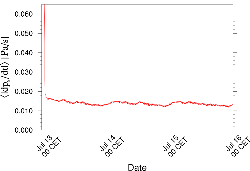
The plot exhibits a high, but rapidly decaying noise level during the first couple of minutes of the model run. The initial noise emerges from spurious imbalances in the initial conditions.
#
Congratulations! You have successfully completed Exercise 2.
Further Reading and Resources#
ICON Tutorial, Ch. 5: https://www.dwd.de/DE/leistungen/nwv_icon_tutorial/nwv_icon_tutorial.html
A new draft version of the ICON Tutorial is available here: https://icon-training-2025-scripts-rendering-cc74a6.gitlab-pages.dkrz.de/index.html. It is currently being finalized and will be published soon.Parallelization was not covered in this tutorial exercise. For details, however, there is an optional exercise, see the Jupyter notebook
icon_exercise_parallelization.ipynb
Author info: Deutscher Wetterdienst (DWD) 2025 :: icon@dwd.de. For a full list of contributors, see CONTRIBUTING in the root directory. License info: see LICENSE file.