
ICON Training - Hands-on Session
Exercise 4: Running the ICON-LAM Setup#
This step-by-step exercise will familiarize you with the basic steps to set up and run ICON-LAM on the DKRZ cluster “Levante”.
It covers the following topics:
necessary input data for running ICON-LAM
preparing the ICON-LAM batch job and namelist
ICON dictionaries
running the ICON-LAM batch job
Note: This script is not suited for operational use, it is part of the step-by-step tutorial.
Example Setup
In this exercise we will perform a 48h forecast run with ICON-LAM over Germany, starting at 2021-07-14 00UTC. Further details of the configuration are provided in the table below. The model will be driven by initial and boundary data which come from global ICON forecasts retrieved from DWD’s database. These data were preprocessed in the previous exercise `Pre-Processing for ICON``.
Configuration |
|
|---|---|
mesh size |
6.5 km (R3B8) |
model top height |
22 km |
no. of levels |
65 |
no. of cells (per level) |
37488 |
time step |
60 s |
duration |
48h |
Necessary input data for ICON-LAM#
Running ICON-LAM requires the following set of input files to be available:
horizontal grid file: coordinates and topological index relations between cells, edges and vertices
external parameter file: time invariant fields such as topography, lake depths or soil type
initial conditions: snapshot of an atmospheric state and soil state from which the model is integrated forward in time
lateral boundary conditions: snapshots of the atmospheric state at regular time intervals, which ‘drives’ the model at its lateral boundaries
Please note that a vertical grid file is not required. The vertical grid is constructed during the initialization phase of ICON, based on a set of ICON namelist parameters.
The preparation of these input files has been discussed in more depth in the exercise Pre-Processing for ICON. At this point we assume that all input files are available and located in the following directories:
initial and boundary data:
$SCRATCHDIR/data_lamgrids and external parameter:
/pool/data/ICON/ICON_training/exercise_lam/grids
export SCRATCHDIR=/scratch/${USER::1}/$USER
Inspecting the boundary data files#
cdo sinfov to investigate the content of a lateral boundary file located in $SCRATCHDIR/data_lam.
The cdo command is available as soon as you have loaded the corresponding module with module load cdo.
- How does it differ from the corresponding 'raw' data file in
$SCRATCHDIR/example_data/raw_data?
<your answer>
Solution
module load cdo
cdo sinfov $SCRATCHDIR/data_lam/forcing_ML_20210714T020000Z_lbc.nc
Answer:
horizontally interpolated from R3B7 (13km) to R3B8 (6.5km)
NetCDF format instead of GRIB2 format
How many timesteps are contained in a single file? What is the time interval between two consecutive boundary data files?
Solution
[ ] none
[X] 1
[ ] 4
The time interval between two consecutive boundary data files is 2 hours
Solution
Answer: The number of vertical levels is different
Get vertical levels in a boundary file:
module load cdo
cdo sinfov $SCRATCHDIR/data_lam/forcing_ML_20210715T060000Z_lbc.nc
boundary file: 90 levels
Model: 65 levels (see table above in Section ‘Example Setup’)
Preparing the ICON-LAM run (namelists etc.)#
Execute the following cell in order to set some environment variables that will be used during this exercise.
# base directory for ICON sources and binary:
export ICONDIR=/pool/data/ICON/ICON_training/icon/

# directory with input grids and external data:
export GRIDDIR=/pool/data/ICON/ICON_training/exercise_lam/grids

# directory with initial and boundary data:
export SCRATCHDIR=/scratch/${USER::1}/$USER
export DATADIR=$SCRATCHDIR/data_lam
# Fallback reference initial and boundary data:
#export DATADIR=/pool/data/ICON/ICON_training/exercise_lam/data_lam

# absolute path to directory with plenty of space:
export EXPDIR=$SCRATCHDIR/exercise_lam
export OUTDIR=$EXPDIR

# absolute path to files needed for radiation
export RADDIR=${ICONDIR}/externals/ecrad/data
Copy input data: grids, external parameters, model. The directory for the experiment will be created, if not already there.
if [ ! -d $EXPDIR ]; then
    mkdir -p $EXPDIR
fi
cd ${EXPDIR}

# grid files and external parameter: link to output directory
ln -sf ${GRIDDIR}/iconR*.nc .
ln -sf ${GRIDDIR}/extpar*.nc .

# data files
ln -sf ${DATADIR}/* .

# dictionaries for the mapping: DWD GRIB2 names <-> ICON internal names
ln -sf ${ICONDIR}/run/ana_varnames_map_file.txt .
ln -sf ${GRIDDIR}/../exercise_lam/map_file.latbc .

# For output: Dictionary for the mapping: names specified in the output nml <-> ICON internal names
cp ${ICONDIR}/run/dict.output.dwd dict.output.dwd
Model namelists#
Create ICON master namelist#
ini_datetime_string and end date end_datetime_string.
ndays_restart=60
dt_restart=$((${ndays_restart}*86400))

cat > icon_master.namelist << EOF
&master_nml
 lrestart = .false.
/
&time_nml
 ini_datetime_string = "??????????"
 end_datetime_string = "??????????"
 dt_restart          = $dt_restart       ! dummy value to avoid crashes
/
&master_model_nml
  model_type=1
  model_name="ATMO"
  model_namelist_filename="NAMELIST_NWP"
  model_min_rank=1
  model_max_rank=65536
  model_inc_rank=1
/
EOF
Solution
ini_datetime_string = "2021-07-14T00:00:00"
end_datetime_string = "2021-07-16T00:00:00"
Create the ICON model namelist NAMELIST_NWP#
In the following we build up the ICON namelist NAMELIST_NWP step by step. To do so, we use the UNIX cat command in order to collect individual namelists into a single file (named NAMELIST_NWP).
for a complete list of namelist parameters see Namelist_overview.pdf:
Please make sure that you execute each of the following cells only once!
l_limited_area (grid_nml) and by specifying lateral boundary data. Of course, other namelist settings might need to be adapted as well, in order to make a proper ICON-LAM setup.
- Switch on the limited area mode by setting
l_limited_areaandinit_mode, see Section 6.3 of the ICON Tutorial. - Initial data: Specify the initial data file via
dwdfg_filename. Since we do not make use of additional analysis information from a second data file, remember to setlread_anaaccordingly (see Section 6.3). - Boundary data: Specify the lateral boundary data via
latbc_filename. You will have to make use of the keywords<y>,<m><d>and<h>(see Section 6.4.1 of the ICON Tutorial).
cat > NAMELIST_NWP << EOF
! grid_nml: horizontal grid --------------------------------------------------
&grid_nml
 dynamics_grid_filename      =       'iconR3B08_DOM01.nc'         ! array of the grid filenames for the dycore
 radiation_grid_filename     =       'iconR3B07_DOM00.nc'         ! array of the grid filenames for the radiation model
 lredgrid_phys               =               .TRUE.,.TRUE.        ! .true.=radiation is calculated on a reduced grid
 lfeedback                   =                      .TRUE.        ! specifies if feedback to parent grid is performed
 ifeedback_type              =                          2         ! feedback type (incremental/relaxation-based)
 l_limited_area              =                 ??????????         ! limited area run TRUE/FALSE
/

! initicon_nml: specify read-in of initial state ------------------------------
&initicon_nml
 init_mode                  =                  ??????????        ! start from DWD initialized analysis
 dwdfg_filename             =                  ??????????        ! initialized analysis data input filename
 lread_ana                  =                  ??????????        ! Read separate analysis file in addition to dwdfg_filename
 ltile_coldstart            =                       .TRUE.       ! coldstart for surface tiles
 ltile_init                 =                      .FALSE.       !
 lp2cintp_sfcana            =                       .TRUE.       ! interpolate surface analysis from global domain onto nest
 ana_varnames_map_file      =   'ana_varnames_map_file.txt'      ! dictionary mapping internal names onto GRIB2 or NetCDF shortNames
/

&limarea_nml
 dtime_latbc                 =                      7200.        ! Time difference between two consecutive boundary data
 init_latbc_from_fg          =                     .TRUE.        ! If .TRUE., take lateral boundary conditions for initial time from FG
 itype_latbc                 =                         1         ! Type of lateral boundary nudging
 latbc_boundary_grid         =                         ''        ! Grid file defining the lateral boundary
 latbc_varnames_map_file     =           'map_file.latbc'        ! dictionary mapping internal names onto GRIB2 or NetCDF shortNames
 latbc_path                  =                       './'        ! path to boundary data
 latbc_filename              =                 ??????????        ! Filename of boundary data input file in the latbc_path directory.
/
EOF
Solution
&grid_nml
 l_limited_area          = .TRUE.
/
&initicon_nml
 init_mode               = 7
 dwdfg_filename          = 'init_ML_20210714T000000Z.nc'
 lread_ana               = .false.
/

&limarea_nml
 latbc_filename          = 'forcing_ML_<y><m><d>T<h>0000Z_lbc.nc'
/
Excursion: ICON dictionaries#
ICON makes use of dictionaries during input and output. A dictionary has the purpose to translate the variable names in the GRIB2 or NetCDF input file into the ICON internal variable names (and vice versa). There exist four different dictionaries, i.e.
ana_varnames_map_filein the namelistiniticon_nml: maps the variable names in the initial conditions file to the ICON internal nameslatbc_varnames_map_filein the namelistlimarea_nml: maps the variable names in the lateral boundary files (LAM) to the ICON internal namesoutput_nml_dictin the namelistio_nml: maps output variable names specified in theoutput_nmlto the ICON internal namesnetcdf_dictin the namelistio_nml: mapping from internal names to names written to the NetCDF file
ana_varnames_map_file.txt (initicon_nml), which is used in this exercise when reading the initial conditions.
According to the dictionary, what are the internal variable names and the GRIB2/NetCDF variable names for
| Variable | GRIB2/NetCDF | ICON internal |
|---|---|---|
| Pressure | ??? | ??? |
| Temperature | ??? | ??? |
| Half level height | ??? | ??? |
- under which conditions does the dictionary
ana_varnames_map_file.txtbecome obsolete (i.e. which conditions must be fulfilled by the initial conditions file)?
Solution
| Variable | GRIB2/NetCDF | ICON internal |
|---|---|---|
| Pressure | P |
pres |
| Temperature | T |
temp |
| Half level height | HHL |
z_ifc |
The dictionary ana_varnames_map_file becomes obsolete, if
the initial conditions are provided in NetCDF format
the NetCDF variable names are equivalent to the ICON internal variable names
Now we add the remaining namelist settings.
For a complete list see Namelist_overview.pdf
cat >> NAMELIST_NWP << EOF
! parallel_nml: MPI parallelization -------------------------------------------
¶llel_nml
nproma = 32 ! loop chunk length
p_test_run = .FALSE. ! .TRUE. means verification run for MPI parallelization
num_io_procs = 1 ! number of I/O processors
num_restart_procs = 0 ! number of restart processors
num_prefetch_proc = 1 ! number of processors for boundary data prefetching
iorder_sendrecv = 3 ! sequence of MPI send/receive calls
num_dist_array_replicas = 4 ! distributed arrays: no. of replications
use_omp_input = .TRUE. ! allows task parallelism for reading atmospheric input data
/
! io_nml: general switches for model I/O -------------------------------------
&io_nml
dt_diag = 21600.0 ! diagnostic integral output interval
dt_checkpoint = 864000.0 ! time interval for writing restart files.
itype_pres_msl = 5 ! method for computation of mean sea level pressure
itype_rh = 1 ! (1) 2: mixed phase (water and ice)
output_nml_dict = 'dict.output.dwd' ! maps output_nml variable names onto internal ICON names
lflux_avg = .TRUE. ! fluxes are accumulated rather than averaged for output
lmask_boundary = .TRUE. ! mask interpolation zone
/
! run_nml: general switches ---------------------------------------------------
&run_nml
num_lev = 65 ! number of full levels (atm.) for each domain
lvert_nest = .FALSE. ! vertical nesting
dtime = 60. ! timestep in seconds
ltestcase = .FALSE. ! idealized testcase runs
ldynamics = .TRUE. ! compute adiabatic dynamic tendencies
ltransport = .TRUE. ! compute large-scale tracer transport
lart = .FALSE. ! ICON-ART main switch
ntracer = 5 ! number of advected tracers
iforcing = 3 ! forcing of dynamics and transport by parameterized processes
msg_level = 11 ! controls how much printout is written during runtime
ltimer = .TRUE. ! timer for monitoring the runtime of specific routines
timers_level = 10 ! performance timer granularity
output = "nml" ! main switch for enabling/disabling components of the model output
/
! nwp_phy_nml: switches for the physics schemes ------------------------------
&nwp_phy_nml
inwp_gscp = 2 ! cloud microphysics (incl. graupel) and precipitation
inwp_convection = 1 ! convection
lshallowconv_only = .FALSE. !
lgrayzone_deepconv = .TRUE. !
inwp_radiation = 4 ! radiation
inwp_cldcover = 1 ! cloud cover scheme for radiation
inwp_turb = 1 ! vertical diffusion and transfer
inwp_satad = 1 ! saturation adjustment
inwp_sso = 1 ! subgrid scale orographic drag
inwp_gwd = 0 ! non-orographic gravity wave drag
inwp_surface = 1 ! surface scheme
latm_above_top = .TRUE. ! take into account atmosphere above model top for radiation computation
ldetrain_conv_prec = .TRUE. !
efdt_min_raylfric = 7200.0 ! minimum e-folding time of Rayleigh friction
itype_z0 = 2 ! type of roughness length data
icapdcycl = 3 ! apply CAPE modification to improve diurnalcycle over tropical land
icpl_aero_conv = 1 ! coupling between autoconversion and Tegen aerosol climatology
icpl_aero_gscp = 1 ! coupling between autoconversion and Tegen aerosol climatology
icpl_o3_tp = 1 ! coupling between ozone mixing ratio and thermal tropopause
dt_rad = 720 ! time step for radiation in s
dt_conv = 120 ! time step for convection in s (domain specific)
dt_sso = 120 ! time step for SSO parameterization
dt_gwd = 120 ! time step for gravity wave drag parameterization
mu_rain = 0.5 ! shape parameter in gamma distribution for rain
rain_n0_factor = 0.1 ! tuning factor for intercept parameter of raindrop size distr.
/
&nwp_tuning_nml
itune_albedo = 1
tune_box_liq_asy = 4.0
tune_gfrcrit = 0.333
tune_gkdrag = 0.125
tune_gkwake = 0.25
tune_gust_factor = 7.0
itune_gust_diag = 3
tune_gustsso_lim = 20.
tune_minsnowfrac = 0.3
tune_sgsclifac = 1.0
tune_rcucov = 0.075
tune_rhebc_land = 0.825
tune_zvz0i = 0.85
icpl_turb_clc = 2
max_calibfac_clcl = 2.0
tune_box_liq = 0.04
tune_eiscrit = 7.
/
! turbdiff_nml: turbulent diffusion -------------------------------------------
&turbdiff_nml
tkhmin = 0.5 ! scaling factor for minimum vertical diffusion coefficient
tkhmin_strat = 0.75 ! Scaling factor for stratospheric minimum vertical diffusion coefficient
tkmmin = 0.75 ! scaling factor for minimum vertical diffusion coefficient
tkmmin_strat = 4.0 ! Scaling factor for stratospheric minimum vertical diffusion coefficient
tur_len = 300. ! Asymptotic maximal turbulent distance
pat_len = 750.0 ! effective length scale of thermal surface patterns
q_crit = 2.0 ! critical value for normalized super-saturation
rat_sea = 0.8 ! controls laminar resistance for sea surface
ltkesso = .TRUE. ! consider TKE-production by sub-grid SSO wakes
frcsmot = 0.2 ! these 2 switches together apply vertical smoothing of the TKE source terms
imode_frcsmot = 2 ! in the tropics (only), which reduces the moist bias in the tropical lower troposphere
imode_tkesso = 2 ! mod of calculating the SSO source term for TKE production
itype_sher = 2 ! type of shear forcing used in turbulence
ltkeshs = .TRUE. ! include correction term for coarse grids in hor. shear production term
a_hshr = 1.25 ! length scale factor for separated horizontal shear mode
alpha1 = 0.125 ! Scaling parameter for molecular roughness of ocean waves
icldm_turb = 2 ! mode of cloud water representation in turbulence
rlam_heat = 10.0 ! Scaling factor of the laminar boundary layer for heat
/
! lnd_nml: land scheme switches -----------------------------------------------
&lnd_nml
ntiles = 3 ! number of tiles
nlev_snow = 3 ! number of snow layers
lmulti_snow = .FALSE. ! .TRUE. for use of multi-layer snow model
idiag_snowfrac = 20 ! type of snow-fraction diagnosis
lsnowtile = .TRUE. ! .TRUE.=consider snow-covered and snow-free separately
itype_canopy = 2 ! Type of canopy parameterization
itype_root = 2 ! root density distribution
itype_trvg = 3 ! BATS scheme with add. prog. var. for integrated plant transpiration since sunrise
itype_evsl = 4 ! type of bare soil evaporation
itype_heatcond = 3 ! type of soil heat conductivity
itype_lndtbl = 4 ! table for associating surface parameters
itype_snowevap = 3 ! Snow evap. in vegetated areas with add. variables for snow age and max. snow height
cwimax_ml = 5.e-4 ! scaling parameter for maximum interception parameterization
c_soil = 1.25 ! surface area density of the (evaporative) soil surface
c_soil_urb = 0.5 ! surface area density of the (evaporative) soil surface, urban areas
lseaice = .TRUE. ! .TRUE. for use of sea-ice model
llake = .TRUE. ! .TRUE. for use of lake model
lprog_albsi = .TRUE. ! sea-ice albedo is computed prognostically
sstice_mode = 2 ! SST is updated by climatological increments on a daily basis
/
! radiation_nml: radiation scheme ---------------------------------------------
&radiation_nml
irad_o3 = 79 ! ozone climatology
irad_aero = 6 ! aerosols
islope_rad = 0 ! slope correction for surface radiation
albedo_type = 2 ! type of surface albedo
albedo_whitecap = 1 ! Ocean albedo increase by foam
direct_albedo_water = 3 ! Direct beam surface albedo over water
vmr_co2 = 425.e-06 ! values representative for 2023
vmr_ch4 = 1900.e-09
vmr_n2o = 334.0e-09
vmr_o2 = 0.20946
vmr_cfc11 = 220.e-12
vmr_cfc12 = 490.e-12
ecrad_data_path = "${RADDIR}" ! Path to folder containing ecRad optical property files
/
! nonhydrostatic_nml: nonhydrostatic model -----------------------------------
&nonhydrostatic_nml
iadv_rhotheta = 2 ! advection method for rho and rhotheta
ivctype = 2 ! type of vertical coordinate
itime_scheme = 4 ! time integration scheme
ndyn_substeps = 5 ! number of dynamics steps per fast-physics step
exner_expol = 0.333 ! temporal extrapolation of Exner function
vwind_offctr = 0.2 ! off-centering in vertical wind solver
damp_height = 12250. ! height at which Rayleigh damping of vertical wind starts
rayleigh_coeff = 5.0 ! Rayleigh damping coefficient
divdamp_order = 24 ! order of divergence damping
divdamp_type = 32 ! type of divergence damping
divdamp_fac = 0.004 ! scaling factor for divergence damping
igradp_method = 3 ! discretization of horizontal pressure gradient
l_zdiffu_t = .TRUE. ! specifies computation of Smagorinsky temperature diffusion
thslp_zdiffu = 0.02 ! slope threshold (temperature diffusion)
thhgtd_zdiffu = 125.0 ! threshold of height difference (temperature diffusion)
htop_moist_proc = 22500.0 ! max. height for moist physics
hbot_qvsubstep = 22500.0 ! height above which QV is advected with substepping scheme
/
! sleve_nml: vertical level specification -------------------------------------
&sleve_nml
min_lay_thckn = 20.0 ! layer thickness of lowermost layer
stretch_fac = 0.65 ! stretching factor to vary distribution of model levels
decay_scale_1 = 4000.0 ! decay scale of large-scale topography component
decay_scale_2 = 2500.0 ! decay scale of small-scale topography component
decay_exp = 1.2 ! exponent of decay function
flat_height = 16000.0 ! height above which the coordinate surfaces are flat
itype_laydistr = 1 ! Type of analytical function to specify the distr. of vert. coords
top_height = 22000.0 ! height of model top
/
! dynamics_nml: dynamical core -----------------------------------------------
&dynamics_nml
iequations = 3 ! type of equations and prognostic variables
divavg_cntrwgt = 0.50 ! weight of central cell for divergence averaging
lcoriolis = .TRUE. ! Coriolis force
/
! transport_nml: tracer transport ---------------------------------------------
&transport_nml
ivadv_tracer = 3, 3, 3, 3, 3, 3 ! tracer specific method to compute vertical advection
itype_hlimit = 3, 4, 4, 4, 4, 4 ! type of limiter for horizontal transport
ihadv_tracer = 52, 2, 2, 2, 2, 3 ! tracer specific method to compute horizontal advection
llsq_svd = .TRUE. ! use QR decomposition for least squares design matrix
beta_fct = 1.005 ! limiter: boost factor for range of permissible values
/
! diffusion_nml: horizontal (numerical) diffusion ----------------------------
&diffusion_nml
lhdiff_vn = .TRUE. ! diffusion on the horizontal wind field
lhdiff_temp = .TRUE. ! diffusion on the temperature field
hdiff_order = 5 ! order of nabla operator for diffusion
itype_vn_diffu = 1 ! reconstruction method used for Smagorinsky diffusion
itype_t_diffu = 2 ! discretization of temperature diffusion
hdiff_efdt_ratio = 24.0 ! ratio of e-folding time to time step
hdiff_smag_fac = 0.025 ! scaling factor for Smagorinsky diffusion
/
! interpol_nml: settings for internal interpolation methods ------------------
&interpol_nml
nudge_zone_width = 10 ! Total width (in units of cell rows) for lateral boundary nudging zone
nudge_max_coeff = 0.075 ! Maximum relaxation coefficient for lateral boundary nudging
lsq_high_ord = 3 ! least squares polynomial order
support_baryctr_intp = .FALSE. !.TRUE. ! .TRUE.: barycentric interpolation support for output
/
! gridref_nml: grid refinement settings --------------------------------------
&gridref_nml
denom_diffu_v = 150. ! denominator for lateral boundary diffusion of velocity
/
! extpar_nml: external data --------------------------------------------------
&extpar_nml
itopo = 1 ! topography (0:analytical)
itype_lwemiss = 2 ! requires updated extpar data
itype_vegetation_cycle = 1 ! specifics for annual cycle of LAI
extpar_filename = 'extpar_DOM<idom>.nc' ! filename of external parameter input file
n_iter_smooth_topo = 1 ! iterations of topography smoother
heightdiff_threshold = 2250. ! threshold above which additional nabla2 diffuion is applied
hgtdiff_max_smooth_topo = 750. ! see Namelist doc
read_nc_via_cdi = .TRUE. ! read NetCDF input data via CDI library
/
&output_nml
! ----------------------------------------------- !
! --- ICON-LAM: output fields - lat/lon grid --- !
! ----------------------------------------------- !
filetype = 4 ! output format: 2=GRIB2, 4=NETCDFv2
dom = 1 ! write lam domain
output_time_unit = 1 ! 1: seconds
output_bounds = 0., 10000000., 3600. ! start, end, increment [s]
steps_per_file = 1
mode = 1 ! 1: forecast mode (relative t-axis), 2: climate mode (absolute t-axis)
include_last = .true.
output_filename = '$OUTDIR/ilfff' ! file name base
filename_format = '<output_filename><ddhhmmss><levtype>'
ml_varlist = 'pres_sfc', 'rh_2m', 't_2m', 'tqv_dia', 'tqc_dia', 'gust10', 'tot_prec', 'asodird_s', 'cape', 'alhfl_s', 'ashfl_s'
remap = 1 ! 0: icon grid, 1: lat-lon
reg_lon_def = 1.0, 0.05, 16.6
reg_lat_def = 44.1, 0.05, 57.5
/
EOF
The ICON-LAM batch job#
The ICON-LAM batch job shown below summarizes all steps which are necessary for running ICON-LAM on the DKRZ Levante platform. Here we assume that all mandatory input fields are available.
cat > $EXPDIR/icon-lam.sbatch << 'EOF'
#!/bin/bash
#SBATCH --job-name=LAM_test
#SBATCH --partition=compute
#SBATCH --nodes=4
#SBATCH --ntasks-per-node=128
#SBATCH --output=slurm.%j.out
#SBATCH --exclusive
#SBATCH --mem-per-cpu=960
#SBATCH --time=00:15:00

### ENV ###
env
set -xe

unset SLURM_EXPORT_ENV
unset SLURM_MEM_PER_NODE
unset SBATCH_EXPORT


# limit stacksize ... adjust to your programs need
# and core file size
ulimit -s 204800
ulimit -c 0
ulimit -l unlimited

export SLURM_DIST_PLANESIZE="32"
export OMPI_MCA_btl="self"
export OMPI_MCA_coll="^ml,hcoll"
export OMPI_MCA_io="romio321"
export OMPI_MCA_osc="ucx"
export OMPI_MCA_pml="ucx"
export UCX_HANDLE_ERRORS="bt"
export UCX_TLS="shm,dc_mlx5,dc_x,self"
export UCX_UNIFIED_MODE="y"
export MALLOC_TRIM_THRESHOLD_="-1"
export OMPI_MCA_pml_ucx_opal_mem_hooks=1

export OMP_NUM_THREADS=1

module load eccodes
export ECCODES_DEFINITION_PATH=/pool/data/ICON/ICON_training/eccodes/definitions.edzw-2.27.0-1:$ECCODES_DEFINITION_PATH

export MODEL=$ICONDIR/build/bin/icon

srun -l --cpu_bind=verbose --hint=nomultithread --distribution=block:cyclic $MODEL

EOF
Submit the job to the HPC cluster, using the Slurm command sbatch.
export ICONDIR=$ICONDIR
cd $EXPDIR && sbatch --account=$SLURM_JOB_ACCOUNT icon-lam.sbatch
Solution
Exercise: 4 nodes with 512 mpi tasks
output_nml_dict = 'dict.output.dwd' (namelist io_nml).ml_varlist = 'pres_sfc', 'rh_2m', 't_2m', 'tqv_dia', 'tqc_dia', 'gust10', 'tot_prec', 'asodird_s', 'cape', 'alhfl_s', 'ashfl_s'
In some cases, e.g. for operational forecast runs, it turned out to be beneficial to use GRIB2 shortnames rather than ICON internal variable names for specifying the output variables.
Try to make use of the dictionary as follows:
- in the
ml_varlist, replace the ICON internal variable names by the corresponding DWD GRIB2 shortnames (see Table A in the ICON tutorial book, Appendix A, for the GRIB2 shortnames) - add missing dictionary entries to
dict.output.dwdin$EXPDIR - Re-run the model, in order to check if the dictionary works. If your dictionary is wrong or incomplete, you will get a runtime error.
Solution
ml_varlist = 'PS', 'RELHUM_2M', 'T_2M', 'TQV_DIA', 'TQC_DIA', 'VMAX_10M', 'TOT_PREC', 'ASWDIR_S', 'CAPE_CON', 'ALHFL_S', 'ASHFL_S'

Additional dictionary entries:

## GRIB2 shortName   internal name
ASWDIR_S             asodird_s
CAPE_CON             cape
Visualizing the model output (the Ahr valley flood)#
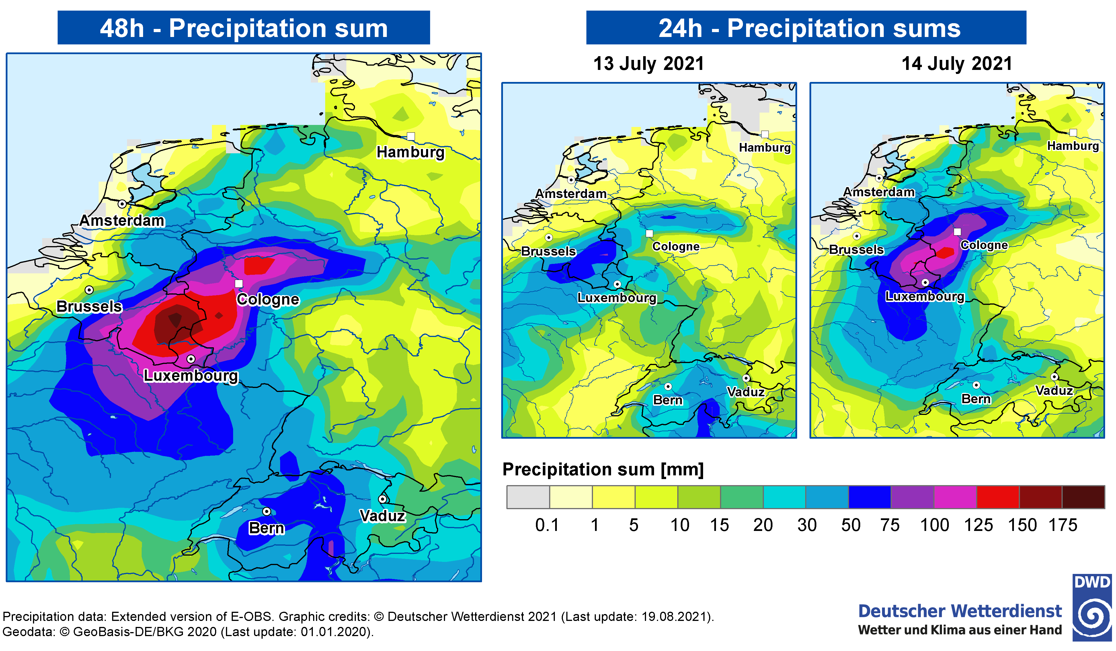
As some of you might have recognized already, the chosen forecast date coincides with the date of the Ahr valley flood event. This heavy rainfall event occurred on July 14-15 near the boarder of Germany and Belgium and tragically caused many fatalities and significant damage to the infrastructure. The observed accumulated precipitation during that period is depicted in the figure to the right.
An in-depth analysis of this event is, of course, beyond the scope of this exercise. However, we will have a look into our forecast result and check, if our very simplified setup was already capable of catching the flood event. To this end, we will visualize the simulated precipitation in our LAM domain and compare with the observations.
Please check if the batch job queue is empty (squeue). Alternatively, you may have a final look at the ICON-LAM log output, to check if the run has finished successfully.
To do so, please navigate to your experiment directory $EXPDIR and open the file slurm.<job_id>.out.
|
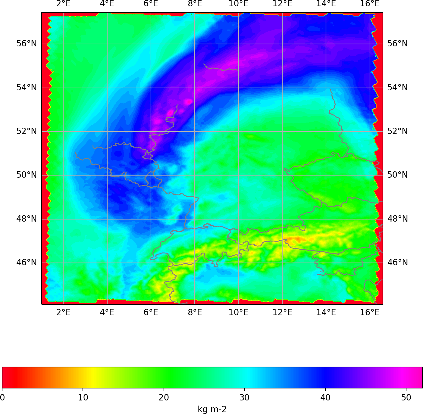
Exercise (Visualization):
Visualize the total column integrated water vapour and cloud water by running the script scripts/icon_exercise_lam_plot_tqv.ipynb. You may adapt the script in order to visualize different dates. |
|
Temporal Resolution of the Boundary Data#
By changing the temporal resolution of your boundary data, you will get some idea how this might affect the quality of your simulation results.
We suggest to create a copy of your experiment directory $EXPDIR, named ${EXPDIR}_orig, in order to avoid overwriting your previous results. To do so, please execute the following cell:
cp -r ${EXPDIR} ${EXPDIR}_orig
- Halve the time resolution of your forcing (boundary) data, see Section 6.4 of the ICON Tutorial for the namelist parameter. Write down the namelist parameter and your chosen value.
${EXPDIR}/NAMELIST_NWP manually in a terminal.
Solution
Answer:
Namelist parameter:
dtime_latbc(limarea_nml)old value: 7200 new value: 14400s
Submit the job to the HPC cluster, using the Slurm command sbatch.
export ICONDIR=$ICONDIR
cd $EXPDIR && sbatch --account=$SLURM_JOB_ACCOUNT icon-lam.sbatch
- Compare the results with your previous run. Does the boundary update frequency have a significant impact on the results?
Congratulations! You have successfully completed Exercise 4.
Further Reading and Resources#
ICON Tutorial: https://www.dwd.de/DE/leistungen/nwv_icon_tutorial/nwv_icon_tutorial.html
A new draft version of the ICON Tutorial is available here: https://icon-training-2025-scripts-rendering-cc74a6.gitlab-pages.dkrz.de/index.html. It is currently being finalized and will be published soon.
Author info: Deutscher Wetterdienst (DWD) 2025 :: icon@dwd.de. For a full list of contributors, see CONTRIBUTING in the root directory. License info: see LICENSE file.