
ICON Training - Hands-on Session
Exercise 1: Running Idealized Test Cases#
The course exercises revisit the topics of the individual tutorial chapters and range from easy tests to the setup of complex forecast simulations. In this particular exercise you will learn how to set up idealized runs in ICON with and without nested domains.
It covers the following topics:
setting up an idealized test case
downloading predefined ICON grids from the ICON download server
running ICON with one or more nested domains
working with the ICON namelist
writing output to disk
Note: This script is not suited for operational use, it is part of the step-by-step tutorial. This exercise focuses on command-line tools and the rudimentary visualization with Python scripts. Professional post-processing and viz tools are beyond the scope of this tutorial.
Necessary input data#
ICON provides a set of predefined test cases of varying complexity and focus, ranging from
pure dynamical core and transport test cases to “moist” cases, including microphysics and
potentially other parameterizations.
If you are interested in more details, please see Chapter 4 of the ICON tutorial (see the link at the bottom of the page).
Most of these tests require only a very limited set of input data, which makes them comparatively easy to set up and run. A graphical overview of the necessary input data is given in the figure below.
Required#
horizontal grid file(s): coordinates and topological index relations between cells, edges and vertices
Not required#
vertical grid file: it is constructed during the initialization phase of ICON
initial condition file: initial conditions are computed by the ICON model itself on the basis of analytical functions.
external parameter file: topography is specified by an analytical function
Jablonowski-Williamson (JW) baroclinic wave test case#
|
The global JW test has become a standard test case for assessing the
quality of atmospheric dynamical cores. |
|
We will set up the JW baroclinic wave test in ICON, first without nested domains:
# base directory for ICON sources and binary:
export ICONDIR=/pool/data/ICON/ICON_training/icon/

# directory with input grids:
export GRIDDIR=$HOME/icon-training-scripts/exercise_idealized/input/

# absolute path to directory with plenty of space:
export SCRATCHDIR=/scratch/${USER::1}/$USER
export EXPDIR=$SCRATCHDIR/exercise_idealized/exp_JW_R02B04

# visualization settings
export SCRIPTDIR=$HOME/icon-training-scripts/exercise_idealized/plot_scripts
In the above settings we used the scratch partition of the file system, with a quota of 15 TiB (see /sw/bin/lfsquota.sh -u $USER).
Retrieve the horizontal grids#
- Open the download page for the predefined ICON grids [weblink] in your web browser.
- Pick the R2B04 grid no. 54 from the list and right-click on the hyperlink for the NetCDF grid file, then choose "copy link location".
- Download the grid file by typing
wget "link_location"to the directory$GRIDDIR - Repeat these steps for the R2B5 grids no. 55 and 56.
cd $GRIDDIR
wget ...
Solution
cd $GRIDDIR
wget http://icon-downloads.mpimet.mpg.de/grids/public/edzw/icon_grid_0054_R02B04_G.nc
wget http://icon-downloads.mpimet.mpg.de/grids/public/edzw/icon_grid_0055_R02B05_N.nc
wget http://icon-downloads.mpimet.mpg.de/grids/public/edzw/icon_grid_0056_R02B05_N.nc
- Copy or link the grid files to the experiment directory. The experiment directory, named exp_JW_R02B04 will be created for you automatically, if not already there.
cd $HOME/icon-training-scripts/exercise_idealized
if [ ! -d $EXPDIR ]; then
    mkdir -p $EXPDIR
fi
cd ${EXPDIR}
echo ${EXPDIR}

# grid files: link to output directory
ln -sf ${GRIDDIR}/?????? .
Solution
if [ ! -d $EXPDIR ]; then
    mkdir -p $EXPDIR
fi
cd ${EXPDIR}
echo ${EXPDIR}

# grid files: link to output directory
ln -sf ${GRIDDIR}/icon_grid_00*.nc .
ICON namelists and job script#
ICON uses Fortran namelists in order to control or modify the model behavior.
Two namelist files have to be provided:
the master namelist file (icon_master.namelist)
contains basic settings such as the model name, or the experiment startdate and enddatethe model namelist file (in this exercise named NAMELIST_NWP)
contains model-specific settings, e.g. for the dynamical core, physics parameterizations and output
In the master namelist file (icon_master.namelist) the name of the model namelist file (here NAMELIST_NWP) must be specified via the parameter model_namelist_filename. The content of the master namelist file is read by ICON at model start. Note that the name of the master namelist file (icon_master.namelist) is hardcoded in the model code and must not be changed.
For a complete list of namelist parameters see Namelist_overview.pdf
Default values are set for all namelist parameters, so that you only have to specify values that differ from the default.
Prepare the ICON Namelists#
- in the master namelist file icon_master.namelist below, insert the name of the model namelist file (see the cell further below for its name)
- execute the cell in order to generate the master namelist file
cat > $EXPDIR/icon_master.namelist << EOF

! master_nml: ----------------------------------------------------------------
&master_nml
 lrestart                   =                      .FALSE.        ! .TRUE.=current experiment is resumed
/

! master_model_nml: repeated for each model ----------------------------------
&master_model_nml
 model_type                  =                          1         ! identifies which component to run (atmosphere,ocean,wave,...)
 model_name                  =                      "ATMO"        ! character string for naming this component.
 model_namelist_filename     =                  ??????????        ! file name containing the model namelists
 model_min_rank              =                          1         ! start MPI rank for this model
 model_max_rank              =                      65536         ! end MPI rank for this model
 model_inc_rank              =                          1         ! stride of MPI ranks
/

! time_nml: specification of date and time------------------------------------
&time_nml
 ini_datetime_string         =       "2012-06-01T00:00:00"        ! initial date and time of the simulation
 end_datetime_string         =       "2012-06-13T00:00:00"        ! end date and time of the simulation
/

EOF
Solution
! master_model_nml: repeated for each model ----------------------------------
&master_model_nml
 model_type                  =                          1         ! identifies which component to run (atmosphere,ocean,...)
 model_name                  =                      "ATMO"        ! character string for naming this component.
 model_namelist_filename     =              "NAMELIST_NWP"        ! file name containing the model namelists
- In the model namelist file NAMELIST_NWP below, fill in the missing namelist parameters.
I.e. setltestcase,ldynamics,iforcing,itopo,dynamics_grid_filenameandnh_test_name.
Hint: The name of the global grid file contains the suffix 'G'.
cat > $EXPDIR/NAMELIST_NWP << EOF
! parallel_nml: MPI parallelization -------------------------------------------
¶llel_nml
nproma = 32 ! loop chunk length
p_test_run = .FALSE. ! .TRUE. means verification run for MPI parallelization
num_io_procs = 1 ! number of I/O processors
num_restart_procs = 0 ! number of restart processors
iorder_sendrecv = 3 ! sequence of MPI send/receive calls
proc0_shift = 0 ! serves for offloading I/O to the vector hosts of the NEC Aurora
use_omp_input = .TRUE. ! allows task parallelism for reading atmospheric input data
/
! run_nml: general switches ---------------------------------------------------
&run_nml
ltestcase = ?????????? ! idealized testcase runs
num_lev = 40 ! number of full levels (atm.) for each domain
lvert_nest = .FALSE. ! vertical nesting
dtime = 1440. ! timestep in seconds
ldynamics = ?????????? ! compute adiabatic dynamic tendencies
ltransport = .FALSE. ! main switch for large-scale tracer transport
ntracer = 0 ! number of advected tracers
iforcing = ?????????? ! pure dynamics (no physics forcing)
msg_level = 10 ! controls how much printout is written during runtime
ltimer = .FALSE. ! timer for monitoring the runtime of specific routines
output = "nml" ! main switch for enabling/disabling components of the model output
/
! diffusion_nml: horizontal (numerical) diffusion ----------------------------
&diffusion_nml
lhdiff_vn = .TRUE. ! diffusion on the horizontal wind field
lhdiff_temp = .TRUE. ! diffusion on the temperature field
lhdiff_w = .TRUE. ! diffusion on the vertical wind field
hdiff_order = 5 ! order of nabla operator for diffusion
itype_vn_diffu = 2 ! reconstruction method used for Smagorinsky diffusion
itype_t_diffu = 2 ! discretization of temperature diffusion
hdiff_efdt_ratio = 20.0 ! ratio of e-folding time to time step
hdiff_smag_fac = 0.02 ! scaling factor for Smagorinsky diffusion
/
! dynamics_nml: dynamical core -----------------------------------------------
&dynamics_nml
iequations = 3 ! type of equations and prognostic variables
divavg_cntrwgt = 0.50 ! weight of central cell for divergence averaging
lcoriolis = .TRUE. ! Coriolis force
/
! extpar_nml: external data --------------------------------------------------
&extpar_nml
extpar_filename = "" ! filename of external parameter input file
itopo = ?????????? ! topography (0:analytical)
n_iter_smooth_topo = 0 ! iterations of topography smoother
/
! grid_nml: horizontal grid --------------------------------------------------
&grid_nml
dynamics_grid_filename = ?????????? ! array of the grid filenames for the dycore
radiation_grid_filename = "" ! array of the grid filenames for the radiation model
lredgrid_phys = .FALSE. ! .true.=radiation is calculated on a reduced grid
lfeedback = .TRUE. ! specifies if feedback to parent grid is performed
ifeedback_type = 2 ! feedback type (incremental/relaxation-based)
/
! sleve_nml: vertical level specification -------------------------------------
&sleve_nml
min_lay_thckn = 20. ! layer thickness of lowermost layer
top_height = 35000. ! height of model top
flat_height = 16000. ! height above which the coordinate surfaces are flat
stretch_fac = 0.9 ! stretching factor to vary distribution of model levels
/
! io_nml: general switches for model I/O -------------------------------------
&io_nml
dt_diag = 21600.0 ! diagnostic integral output interval
dt_checkpoint = 5760000.0 ! time interval for writing restart files.
/
! nh_testcase_nml: idealized testcase specification --------------------------
&nh_testcase_nml
nh_test_name = ?????????? ! testcase selection
jw_up = 1.0 ! amplitude of u-perturbation [m/s]
/
! nonhydrostatic_nml: nonhydrostatic model -----------------------------------
&nonhydrostatic_nml
iadv_rhotheta = 2 ! advection method for rho and rhotheta
ivctype = 2 ! type of vertical coordinate
exner_expol = 0.5 ! temporal extrapolation of Exner function
vwind_offctr = 0.2 ! off-centering in vertical wind solver
damp_height = 25000. ! height at which Rayleigh damping of vertical wind starts
rayleigh_coeff = 0.025 ! Rayleigh damping coefficient
divdamp_fac = 0.0016 ! scaling factor for divergence damping
divdamp_order = 4 ! order of divergence damping
igradp_method = 3 ! discretization of horizontal pressure gradient
l_zdiffu_t = .TRUE. ! specifies computation of Smagorinsky temperature diffusion
thslp_zdiffu = 0.02 ! slope threshold (temperature diffusion)
thhgtd_zdiffu = 125.0 ! threshold of height difference (temperature diffusion)
/
! nwp_phy_nml: switches for the physics schemes ------------------------------
&nwp_phy_nml
inwp_gscp = 0 ! cloud microphysics and precipitation
inwp_convection = 0 ! convection
inwp_radiation = 0 ! radiation
inwp_cldcover = 0 ! cloud cover scheme for radiation
inwp_turb = 0 ! vertical diffusion and transfer
inwp_satad = 0 ! saturation adjustment
inwp_sso = 0 ! subgrid scale orographic drag
inwp_gwd = 0 ! non-orographic gravity wave drag
inwp_surface = 0 ! surface scheme
/
! gridref_nml: switches for grid refinement -----------------------------------
&gridref_nml
denom_diffu_v = 150. ! denominator for lateral boundary diffusion of velocity
fbk_relax_timescale = 43200. ! relaxation time scale for feedback
/
! output_nml: specifies an output stream --------------------------------------
! model level output on native (triangular) grid
&output_nml
filetype = 4 ! output format: 2=GRIB2, 4=NETCDFv2
dom = -1 ! write all domains
output_bounds = 0., 10000000., 43200. ! output: start, end, increment
steps_per_file = 30 ! number of output steps in one output file
mode = 1 ! 1: forecast mode (relative t-axis), 2: climate mode (absolute t-axis)
include_last = .TRUE. ! flag whether to include the last time step
output_filename = 'exp1_JW' ! file name base
output_grid = .TRUE. ! flag whether grid information is added to output.
!
ml_varlist = 'u', 'v', 'w', 'temp', 'pres','topography_c', 'pres_sfc', 'vor', 'div'
/
! output_nml: specifies an output stream --------------------------------------
! pressure level output on native grid
&output_nml
filetype = 4 ! output format: 2=GRIB2, 4=NETCDFv2
dom = -1 ! write all domains
output_bounds = 0., 10000000., 43200. ! output: start, end, increment
steps_per_file = 30 ! number of output steps in one output file
mode = 1 ! 1: forecast mode (relative t-axis), 2: climate mode (absolute t-axis)
include_last = .TRUE. ! flag whether to include the last time step
output_filename = 'exp1_JW' ! file name base
output_grid = .TRUE. ! flag whether grid information is added to output.
remap = 0 ! no remapping (native grid)
!
pl_varlist = 'temp', 'vor', 'div'
p_levels = 50000.,70000.,85000.,92500. ! pressure levels in Pa
/
! output_nml: specifies an output stream --------------------------------------
! model level output on regular lat/lon grid
&output_nml
filetype = 4 ! output format: 2=GRIB2, 4=NETCDFv2
dom = -1 ! write all domains
output_bounds = 0., 10000000., 86400. ! output: start, end, increment
steps_per_file = 30 ! number of output steps in one output file
mode = 1 ! 1: forecast mode (relative t-axis), 2: climate mode (absolute t-axis)
include_last = .TRUE. ! flag whether to include the last time step
output_filename = 'exp1_JW_lonlat' ! file name base
output_grid = .TRUE. ! flag whether grid information is added to output.
remap = 1 ! remap to regular lat/lon grid
reg_lat_def = -90.,1.0,90. ! start, increment, end latitude in degrees
reg_lon_def = 0.,1.0,359.0 ! start, increment, end longitude in degrees
!
ml_varlist = 'u', 'v', 'w', 'temp', 'pres','topography_c', 'pres_sfc', 'vor', 'div'
/
EOF
Solution
&run_nml ltestcase = .TRUE. ! idealized testcase runs ldynamics = .TRUE. ! compute adiabatic dynamic tendencies iforcing = 0 ! pure dynamics (no physics forcing)&extpar_nml itopo = 0 ! topography (0:analytical)&grid_nml dynamics_grid_filename = 'icon_grid_0054_R02B04_G.nc' ! array of the grid filenames for the dycore&nh_testcase_nml nh_test_name = 'jabw' ! testcase selection
Prepare the ICON batch job#
$ICONDIR/build.
The process of building the ICON model will be described in Exercise icon_exercise_programming.ipynb
- In the cell below, specify the path to your ICON model binary (fill in the name of the ICON model binary including the path).
- Create the ICON batch job file icon.sbatch by executing the cell (job will not be submitted to the HPC cluster).
cat > $EXPDIR/icon.sbatch << 'EOF'
#!/bin/bash
#SBATCH --job-name=JW_test
#SBATCH --partition=compute
#SBATCH --nodes=1
#SBATCH --ntasks-per-node=128
#SBATCH --output=slurm.%j.out
#SBATCH --exclusive
#SBATCH --mem-per-cpu=960
#SBATCH --time=00:10:00

### ENV ###
env
set -xe

unset SLURM_EXPORT_ENV
unset SLURM_MEM_PER_NODE
unset SBATCH_EXPORT


# limit stacksize ... adjust to your programs need
# and core file size
ulimit -c 0
ulimit -l unlimited

export OMP_NUM_THREADS=1

# OpenMPI environment settings
export OMPI_MCA_osc="ucx"
export OMPI_MCA_pml="ucx"
export OMPI_MCA_btl="self"
export UCX_HANDLE_ERRORS="bt"
export OMPI_MCA_pml_ucx_opal_mem_hooks=1
export OMPI_MCA_io="romio321"              # basic optimisation of I/O
export UCX_TLS="shm,rc_mlx5,rc_x,self"     # for jobs using LESS than 150 nodes
export UCX_UNIFIED_MODE="y"                # JUST for homogeneous jobs on CPUs, do not use for GPU nodes


# path to model binary, including the executable:
MODEL=??????????

srun -l --cpu_bind=verbose --hint=nomultithread --distribution=block:cyclic $MODEL

EOF
Note: This run script - and likewise the run scripts from the following exercises - contains a whole series of platform-specific settings for parallel execution (e.g. export OMPI_MCA_osc). These are documented for the advanced user under https://docs.dkrz.de/doc/levante/running-jobs/runtime-settings.html#mpi-runtime-settings.
Solution
# path to model binary, including the executable:
MODEL=$ICONDIR/build/bin/icon
All files which are required to run the Jablonowski-Williamson test case have now been generated and stored in $EXPDIR.
Please list the content of $EXPDIR, and remind yourself about the purpose of the individual files.
Solution
icon_grid_0056_R02B05_N.nc icon_grid_0055_R02B05_N.nc icon_grid_0054_R02B04_G.nc icon_master.namelist NAMELIST_NWP icon.sbatch
Running the ICON model#
sbatch.
cd $EXPDIR && sbatch --account=$SLURM_JOB_ACCOUNT icon.sbatch
Checking the job status#
squeue.
Hint: In order to list only jobs belonging to your user ID, you can make use of the option -u $USER
Solution
squeue -u $USER
Inspecting the output#
Open a terminal by clicking the following button and go to the output directory $EXPDIR. You will find three NetCDF output files with
(a) model level output on the native (triangular) grid
(b) pressure level output on the native grid
(c) model level output interpolated onto a regular lat-lon grid.
cdo and ncdump as described in Section 10.1 of the tutorial.
- write down one or more metadata from which the type of horizontal and vertical grid can be inferred
cdo and netcdf-c.
Solution
grid metainformation: ‘height’, ‘plev’, ‘lon’, ‘lat’ (ncdump) or ‘grid coordinates’/’vertical coordinates’ (CDO)
Solution
output interval: 12h (but 24h for lat-lon output) solution: cdo sinfov
pip install matplotlib cartopy xarray netCDF4 'numpy<2'
cd $EXPDIR
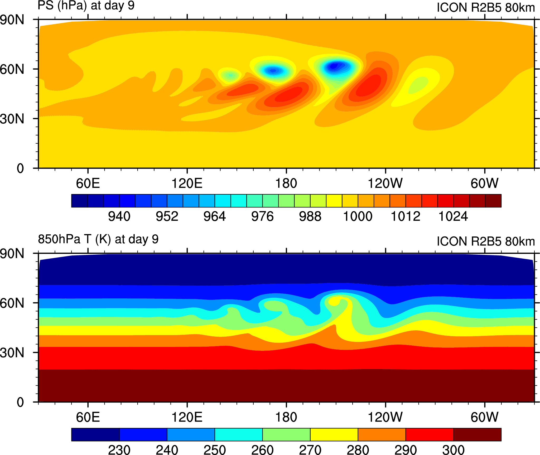
PREFIX="exp1" python3 $SCRIPTDIR/JW_day9_pres_vort_temp_NH_and_SH.py
- Have a closer look at the southern hemisphere. Is the flow in the southern hemisphere still purely zonal after 9 days?
- Describe what you see. Do you have an explanation for the observed behavior?
Solution
Answer:A deviation from the zonally symmetric flow (wavenumber 5 disturbance) becomes apparent after approx. day 5. The disturbance maximum does not occur in the proximity of the pentagon points (\(lat\approx 27\deg\)), but in the region of largest baroclinicity (\(lat\approx 60\deg\)). This deviation from the zonally symmetric flow is not a direct consequence of the existence of the pentagon points but a consequence of the overall grid irregularity (area, angle, etc.) and its periodicity.
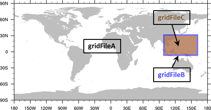
Grid Nesting#
The JW test is well suited to learn about ICON’s nesting capability. We will repeat the previous exercise with one or more additional nested domains. As we will see, activating nested domains reqires only a few namelist changes.
The grid files of the nested domains have already been downloaded by you at the beginning of this exercise (grids no. 55 and 56).
The geographic location of these nests is depicted in the figure below.
Please verify that the grid files are stored in the subdirectory $GRIDDIR and linked (or copied) to the experiment directory $EXPDIR.
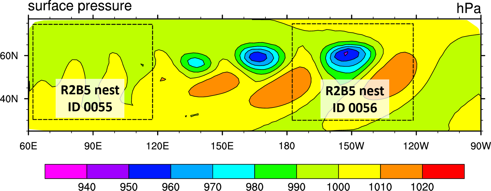
- activate both nested domains by adapting
dynamics_grid_filename (grid_nml) - ensure that the nested domains have the same top height as the global domain, by adapting
num_lev (run_nml)
The same output fields as for the global domain will be generated for the regional domain(s). We will be using the new file prefix exp2, in order to avoid overwriting your previous results
Prepare the ICON Namelist#
cat > $EXPDIR/NAMELIST_NWP << EOF
! parallel_nml: MPI parallelization -------------------------------------------
¶llel_nml
nproma = 32 ! loop chunk length
p_test_run = .FALSE. ! .TRUE. means verification run for MPI parallelization
num_io_procs = 1 ! number of I/O processors
num_restart_procs = 0 ! number of restart processors
iorder_sendrecv = 3 ! sequence of MPI send/receive calls
proc0_shift = 0 ! serves for offloading I/O to the vector hosts of the NEC Aurora
use_omp_input = .TRUE. ! allows task parallelism for reading atmospheric input data
/
! run_nml: general switches ---------------------------------------------------
&run_nml
ltestcase = .TRUE. ! idealized testcase runs
num_lev = 40,?????????? ! number of full levels (atm.) for each domain
lvert_nest = .FALSE. ! vertical nesting
dtime = 1440. ! timestep in seconds
ldynamics = .TRUE. ! compute adiabatic dynamic tendencies
ltransport = .FALSE. ! main switch for large-scale tracer transport
ntracer = 0 ! number of advected tracers
iforcing = 0 ! pure dynamics (no physics forcing)
msg_level = 10 ! controls how much printout is written during runtime
ltimer = .FALSE. ! timer for monitoring the runtime of specific routines
output = "nml" ! main switch for enabling/disabling components of the model output
/
! diffusion_nml: horizontal (numerical) diffusion ----------------------------
&diffusion_nml
lhdiff_vn = .TRUE. ! diffusion on the horizontal wind field
lhdiff_temp = .TRUE. ! diffusion on the temperature field
lhdiff_w = .TRUE. ! diffusion on the vertical wind field
hdiff_order = 5 ! order of nabla operator for diffusion
itype_vn_diffu = 2 ! reconstruction method used for Smagorinsky diffusion
itype_t_diffu = 2 ! discretization of temperature diffusion
hdiff_efdt_ratio = 20.0 ! ratio of e-folding time to time step
hdiff_smag_fac = 0.02 ! scaling factor for Smagorinsky diffusion
/
! dynamics_nml: dynamical core -----------------------------------------------
&dynamics_nml
iequations = 3 ! type of equations and prognostic variables
divavg_cntrwgt = 0.50 ! weight of central cell for divergence averaging
lcoriolis = .TRUE. ! Coriolis force
/
! extpar_nml: external data --------------------------------------------------
&extpar_nml
extpar_filename = "" ! filename of external parameter input file
itopo = 0 ! topography (0:analytical)
n_iter_smooth_topo = 0 ! iterations of topography smoother
/
! grid_nml: horizontal grid --------------------------------------------------
&grid_nml
dynamics_grid_filename = ?????????? ! array of the grid filenames for the dycore
radiation_grid_filename = "" ! array of the grid filenames for the radiation model
lredgrid_phys = .FALSE. ! .true.=radiation is calculated on a reduced grid
lfeedback = .TRUE. ! specifies if feedback to parent grid is performed
ifeedback_type = 2 ! feedback type (incremental/relaxation-based)
dynamics_parent_grid_id = 0,1,1 ! explicit setting of grid hierarchy (needed due to code bug)
/
! sleve_nml: vertical level specification -------------------------------------
&sleve_nml
min_lay_thckn = 20. ! layer thickness of lowermost layer
top_height = 35000. ! height of model top
flat_height = 16000. ! height above which the coordinate surfaces are flat
stretch_fac = 0.9 ! stretching factor to vary distribution of model levels
/
! io_nml: general switches for model I/O -------------------------------------
&io_nml
dt_diag = 21600.0 ! diagnostic integral output interval
dt_checkpoint = 5760000.0 ! time interval for writing restart files.
/
! nh_testcase_nml: idealized testcase specification --------------------------
&nh_testcase_nml
nh_test_name = "jabw" ! testcase selection
jw_up = 1.0 ! amplitude of u-perturbation [m/s]
/
! nonhydrostatic_nml: nonhydrostatic model -----------------------------------
&nonhydrostatic_nml
iadv_rhotheta = 2 ! advection method for rho and rhotheta
ivctype = 2 ! type of vertical coordinate
exner_expol = 0.5 ! temporal extrapolation of Exner function
vwind_offctr = 0.2 ! off-centering in vertical wind solver
damp_height = 25000. ! height at which Rayleigh damping of vertical wind starts
rayleigh_coeff = 0.025 ! Rayleigh damping coefficient
divdamp_fac = 0.0016 ! scaling factor for divergence damping
divdamp_order = 4 ! order of divergence damping
igradp_method = 3 ! discretization of horizontal pressure gradient
l_zdiffu_t = .TRUE. ! specifies computation of Smagorinsky temperature diffusion
thslp_zdiffu = 0.02 ! slope threshold (temperature diffusion)
thhgtd_zdiffu = 125.0 ! threshold of height difference (temperature diffusion)
/
! nwp_phy_nml: switches for the physics schemes ------------------------------
&nwp_phy_nml
inwp_gscp = 0 ! cloud microphysics and precipitation
inwp_convection = 0 ! convection
inwp_radiation = 0 ! radiation
inwp_cldcover = 0 ! cloud cover scheme for radiation
inwp_turb = 0 ! vertical diffusion and transfer
inwp_satad = 0 ! saturation adjustment
inwp_sso = 0 ! subgrid scale orographic drag
inwp_gwd = 0 ! non-orographic gravity wave drag
inwp_surface = 0 ! surface scheme
/
! gridref_nml: switches for grid refinement -----------------------------------
&gridref_nml
denom_diffu_v = 150. ! denominator for lateral boundary diffusion of velocity
fbk_relax_timescale = 43200. ! relaxation time scale for feedback
/
! output_nml: specifies an output stream --------------------------------------
! model level output on native (triangular) grid
&output_nml
filetype = 4 ! output format: 2=GRIB2, 4=NETCDFv2
dom = -1 ! write all domains
output_bounds = 0., 10000000., 43200. ! output: start, end, increment
steps_per_file = 30 ! number of output steps in one output file
mode = 1 ! 1: forecast mode (relative t-axis), 2: climate mode (absolute t-axis)
include_last = .TRUE. ! flag whether to include the last time step
output_filename = 'exp2_JW' ! file name base
output_grid = .TRUE. ! flag whether grid information is added to output.
!
ml_varlist = 'u', 'v', 'w', 'temp', 'pres','topography_c', 'pres_sfc', 'vor', 'div'
/
! output_nml: specifies an output stream --------------------------------------
! pressure level output on native grid
&output_nml
filetype = 4 ! output format: 2=GRIB2, 4=NETCDFv2
dom = -1 ! write all domains
output_bounds = 0., 10000000., 43200. ! output: start, end, increment
steps_per_file = 30 ! number of output steps in one output file
mode = 1 ! 1: forecast mode (relative t-axis), 2: climate mode (absolute t-axis)
include_last = .TRUE. ! flag whether to include the last time step
output_filename = 'exp2_JW' ! file name base
output_grid = .TRUE. ! flag whether grid information is added to output.
remap = 0 ! no remapping (native grid)
!
pl_varlist = 'temp', 'vor', 'div'
p_levels = 50000.,70000.,85000.,92500. ! pressure levels in Pa
/
! output_nml: specifies an output stream --------------------------------------
! model level output on regular lat/lon grid
&output_nml
filetype = 4 ! output format: 2=GRIB2, 4=NETCDFv2
dom = -1 ! write all domains
output_bounds = 0., 10000000., 43200. ! output: start, end, increment
steps_per_file = 30 ! number of output steps in one output file
mode = 1 ! 1: forecast mode (relative t-axis), 2: climate mode (absolute t-axis)
include_last = .TRUE. ! flag whether to include the last time step
output_filename = 'exp2_JW_lonlat' ! file name base
output_grid = .TRUE. ! flag whether grid information is added to output.
remap = 1 ! remap to regular lat/lon grid
reg_lat_def = -90.,1.0,90. ! start, increment, end latitude in degrees
reg_lon_def = 0.,1.0,359.0 ! start, increment, end longitude in degrees
!
ml_varlist = 'u', 'v', 'w', 'temp', 'pres','topography_c', 'pres_sfc', 'vor', 'div'
/
EOF
Solution
&grid_nml dynamics_grid_filename = 'icon_grid_0054_R02B04_G.nc','icon_grid_0055_R02B05_N.nc','icon_grid_0056_R02B05_N.nc'&run_nml num_lev = 40,40,40 ! number of full levels (atm.) for each domain
Running the ICON model#
Submit the job to the HPC cluster, using the Slurm command sbatch.
cd $EXPDIR && sbatch --account=$SLURM_JOB_ACCOUNT icon.sbatch
Check the job status using the Slurm command squeue
#
Inspecting the output#
# set filename prefix
export PREFIX="exp2"
cd $EXPDIR
python3 $SCRIPTDIR/JW_day9_pres_vort_temp_NH_and_SH.py
python3 $SCRIPTDIR/JW_day9_pres_and_vort_merge_2nests.py
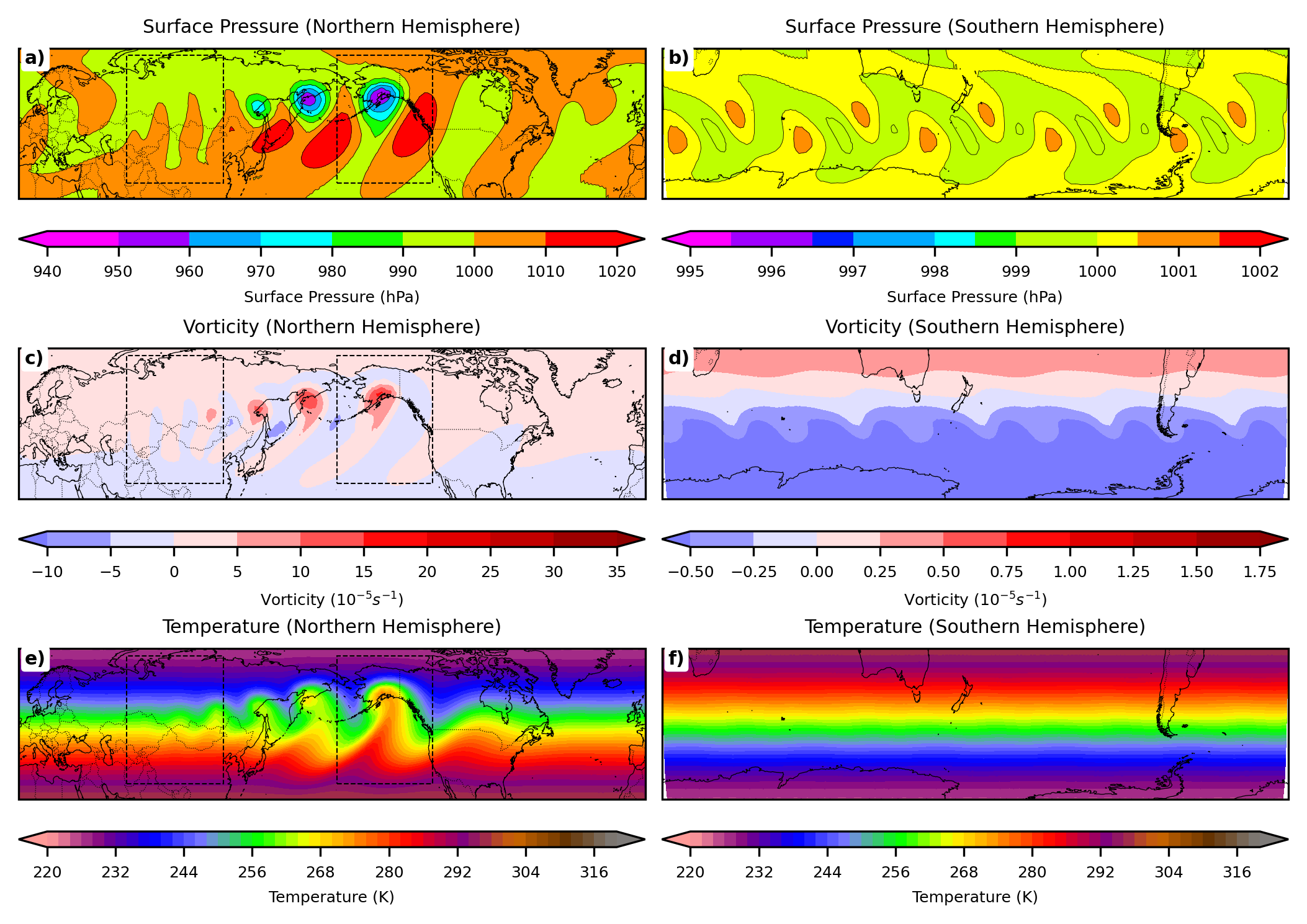
- The first plot [here] shows the results for the global R2B4 domain. Compare your results with the global domain results of the previous exercise.
- Does your result differ?
- If so, do you have an explanation for this?
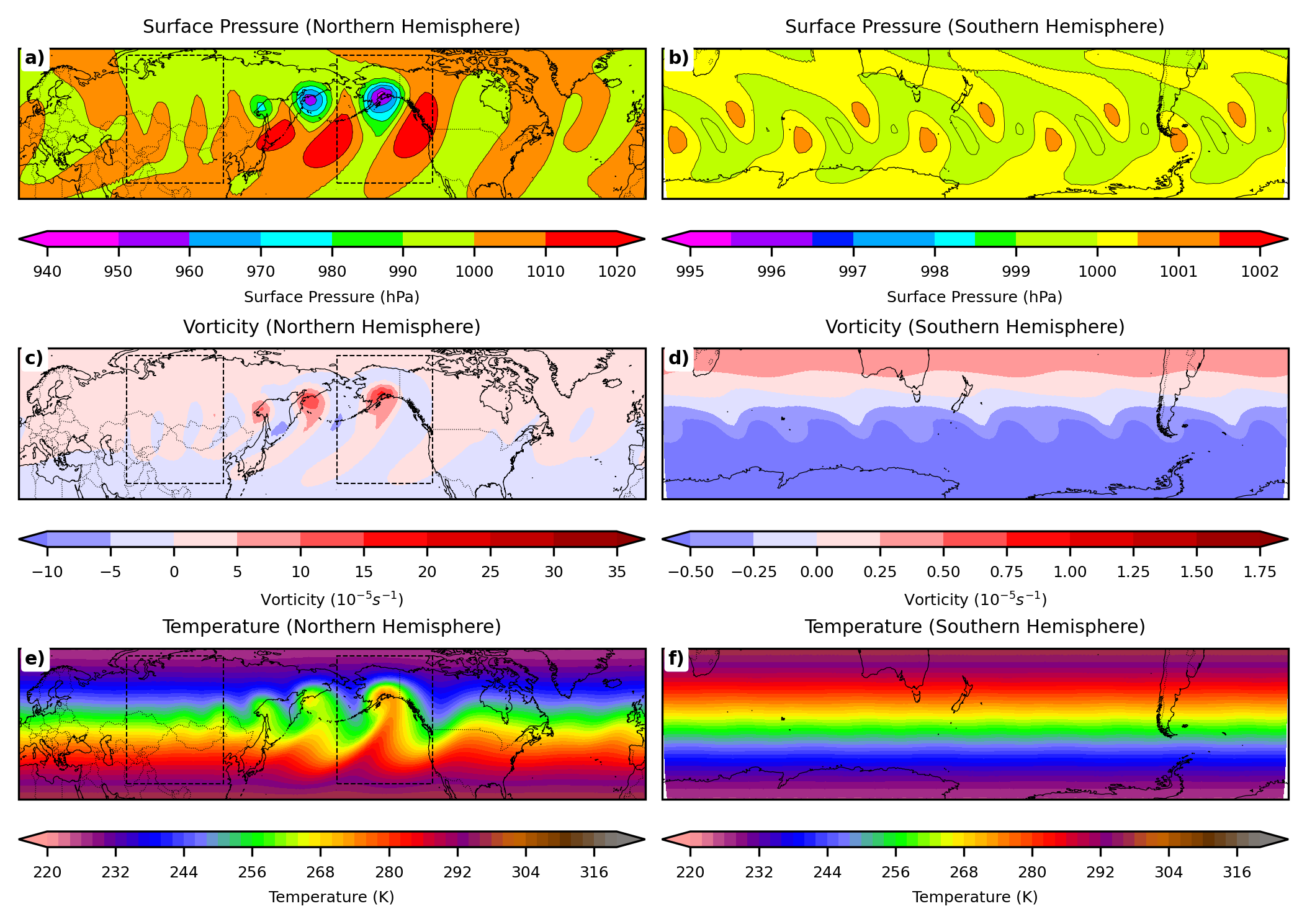
- Have a look at the second plot [here].
- Do you have an idea which solution (in terms of which domain(s)) is shown in this plot? Describe what you see.
![[here]](./exp2_JW_R2B4N5_day9_pres_vort_temp.png)
![[here]](./exp2_JW_day9_pres_and_vort_merged.png)
If you want to verify that your global domain results are correct, you can compare with the global domain reference solution here.
Solution
Answer:- Yes, results on the global domain differ, since the parent to child feedback is switched on (
lfeedback=.TRUE.; see namelistgrid_nml) Comment: Withlfeedback=.FALSE. (grid_nml), the run without nests and the nested runs give identical results for the global domain. Please feel free to run this additional experiment. - The second plot shows the 'combined' solution, which means that the highest-resolution data are shown in any region of the plot.
Parent-child relationships#
|
The figure to the right depicts an alternative configuration using three domains,
in which the two nested domains are consecutively nested into each other (multi-level nesting).
How does ICON know about the actual parent-child relationship of the grids in use? |
|
See Section 3.9, page 121 of the tutorial for an explanation and
- write down the parameters from which the parent-child relationship is inferred.
- open a terminal and try to identify these parameters in your grid files (you might make use of
ncdump)
Solution
Answer: The parent-child information is inferred from NetCDF attributes stored in the grid files. These attributes are
uuidOfHGrid: unique identifier of the current griduuidOfParHGrid: unique identifier of the current grids’ parent grid.
module load netcdf-c
ncdump -h $EXPDIR/icon_grid_0055_R02B05_N.nc | grep "uuidOf"
Congratulations! You have successfully completed Exercise 1.
Further Reading and Resources#
ICON Tutorial, Ch. 4: https://www.dwd.de/DE/leistungen/nwv_icon_tutorial/nwv_icon_tutorial.html
A new draft version of the ICON Tutorial is available here: https://icon-training-2025-scripts-rendering-cc74a6.gitlab-pages.dkrz.de/index.html. It is currently being finalized and will be published soon.Tracer transport was not covered in this tutorial exercise. For details, however, there is an optional exercise, see the Jupyter notebook
icon_exercise_idealized_transport.ipynb
Author info: Deutscher Wetterdienst (DWD) 2025 :: icon@dwd.de. For a full list of contributors, see CONTRIBUTING in the root directory. License info: see LICENSE file.