
ICON Training - Hands-on Session
Optional exercise 2: Parallelization and Run-Time Performance#
The course exercises revisit the topics of the individual tutorial chapters and range from easy tests to the setup of complex forecast simulations.
In this particular exercise you will learn how to
make use of the built-in timer module for performance diagnostic
specify details of the parallel model execution
Note: This script is not suited for operational use, it is part of the step-by-step tutorial. Furthermore, we will omit some of ICON’s less important input and output channels here, e.g. the restart files. This exercise focuses on command-line tools and the rudimentary visualization with Python scripts. Professional post-processing and viz tools are beyond the scope of this tutorial.
Setup#
We will start from the global setup (without nest), which has been used in exercise 2 “Global Real Data Run”.
Configuration |
|
|---|---|
mesh size |
40 km (R2B6) |
model top height |
75 km |
no. of levels |
90 |
no. of cells (per level) |
327680 |
time step |
360 s |
duration |
12h |
All input and configuration files have already been prepared for you. These include
the master namelist (icon_master.namelist)
the model namelist (NAMELIST_NWP)
the ICON batch job file (icon.sbatch)
the horizontal grid and external parameter file
the analysis file.
When executing the two cells below, the experiment directory $EXPDIR will be prepared for you, including all the required files listed above.
# base directory for ICON sources and binary:
ICONDIR=/pool/data/ICON/ICON_training/icon/

# directory with input grids and external data:
GRIDDIR=/pool/data/ICON/ICON_training/exercise_realdata/grids
# directory with initial data:
DATADIR=/pool/data/ICON/ICON_training/exercise_realdata/data/ini

# absolute path to directory with plenty of space:
SCRATCHDIR=/scratch/${USER::1}/$USER
EXPDIR=$SCRATCHDIR/exercise_parallelization

# absolute path to files needed for radiation
RADDIR=${ICONDIR}/externals/ecrad/data

# path to prepared namelists
NMLDIR=/pool/data/ICON/ICON_training/exercise_realdata/setup_global
$EXPDIR: grids, external parameters, initial conditions, namelists.
The directory for the experiment will be created, if not already there.
if [ ! -d $EXPDIR ]; then
    mkdir -p $EXPDIR
fi
cd ${EXPDIR}

# grid files: link to output directory
ln -sf ${GRIDDIR}/iconR*.nc .
# external parameter files: link to output directory
ln -sf ${GRIDDIR}/extpar*.nc .
# data files: link to output directory
ln -sf ${DATADIR}/*.grb .

# Dictionary for the mapping: DWD GRIB2 names <-> ICON internal names
ln -sf ${ICONDIR}/run/ana_varnames_map_file.txt map_file.ana

# For Output: Dictionary for the mapping: names specified in the output nml <-> ICON internal names
ln -sf ${ICONDIR}/run/dict.output.dwd dict.output.dwd

# copy the master namelist, model namelist and job script to the output directory
cp ${NMLDIR}/icon_master.namelist .
cp ${NMLDIR}/NAMELIST_NWP_global NAMELIST_NWP
cp ${NMLDIR}/icon.sbatch .
Measuring the run-time performance#
In this exercise you will learn how to make use of the ICON timer module for basic performance measurement.
- Open an interactive Linux terminal by clicking the following button
- Navigate to your experiment directory
$EXPDIRand open the ICON namelistNAMELIST_NWP - Enable the ICON routines for performance logging (timers).
To do so, follow the instructions in Section 8.4, "Basic Performance Measurement", of the ICON tutorial. - Run the model by submitting the job script
icon.sbatch.
At the end of the model run, a log file slurm.XYZ.out is created. It can be found in your experiment directory $EXPDIR. Scroll to the end of this file. You should find wall clock timer output comparable to that listed in Section 8.4. Try to identify
the total run-time
the time needed by the radiation module
Submit your ICON batch job
export ICONDIR=$ICONDIR
cd $EXPDIR && sbatch icon.sbatch
Check the job status via squeue
Solution
Namelist changes
&run_nml
  ltimer       = .TRUE.
  timers_level = 10
/
Wall clock timer output
- total run-time: ~ 85s
- radiation run-time: ~ 11s
#
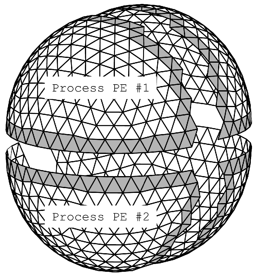
Specifying details of parallel model execution#
The next exercise focuses on the mechanisms for parallel execution of the ICON model. These settings become important for performance scalability, when increasing the model resolution and core counts.
- Modify your batch job script
icon.sbatchinEXPDIRand double the total number of MPI tasks compared to your previous job. You will need to adjust only theSlurmsettings. See Example Batch Scripts for additional help. - In more detail, do the following:
- Your previous script ran the executable on $5$ nodes using $128$ MPI tasks/node and $1$ OpenMP threads/MPI task.
- Your new script should run the executable on $10$ nodes using $128$ MPI tasks/node and $1$ OpenMP threads/MPI task.
- Repeat the model run
Solution
#SBATCH --nodes=10
#SBATCH --ntasks-per-node=128
#
Submit your ICON batch job
export ICONDIR=$ICONDIR
cd $EXPDIR && sbatch icon.sbatch
Check the job status via squeue
#
nh_solve, and the transport module, transport, with the timer output of your previous run.
What do you think is a more sensible measure of the effective cost:
total minortotal max?Compute the speedup that you gained from doubling the number of MPI tasks. Which speedup did you achieve and what would you expect from “theory”?
Speedup achieved \(=\frac{T_{\mathrm{x}}}{T_{\mathrm{2x}}} = \ldots\)
Sensible measure of effective cost …
Solution
Answer:
Sensible measure of effective cost: total max (processes are typically waiting for the slowest one at barriers)
approximate speedup: nh_solve: 46.5s/24.9s = 1.87; transport: 10.1s/5.4s = 1.87
theoretical expectation: speedup factor 2
grid |
namelist parameter |
|---|---|
dynamics grid(s) |
|
radiation grid: |
|
#
Congratulations! You have successfully completed optional Exercise 2.
Further Reading and Resources#
ICON Tutorial, Ch. 5: https://www.dwd.de/DE/leistungen/nwv_icon_tutorial/nwv_icon_tutorial.html
A new draft version of the ICON Tutorial is available here: https://icon-training-2025-scripts-rendering-cc74a6.gitlab-pages.dkrz.de/index.html. It is currently being finalized and will be published soon.
Author info: Deutscher Wetterdienst (DWD) 2025 :: icon@dwd.de. For a full list of contributors, see CONTRIBUTING in the root directory. License info: see LICENSE file.